Monday, October 31, 2016

The Alien Blaster Problem

Last week I posted the Alien Blaster Problem:

In preparation for an alien invasion, the Earth Defense League has been working on new missiles to shoot down space invaders.  Of course, some missile designs are better than others; let's assume that each design has some probability of hitting an alien ship, x.

Based on previous tests, the distribution of x in the population of designs is roughly uniform between 10% and 40%.  To approximate this distribution, we'll assume that x is either 10%, 20%, 30%, or 40% with equal probability.

Now suppose the new ultra-secret Alien Blaster 10K is being tested.  In a press conference, an EDF general reports that the new design has been tested twice, taking two shots during each test.  The results of the test are confidential, so the general won't say how many targets were hit, but they report: ``The same number of targets were hit in the two tests, so we have reason to think this new design is consistent.''

Is this data good or bad; that is, does it increase or decrease your estimate of x for the Alien Blaster 10K?

Now here's a solution:


I'll start by creating a Pmf that represents the four hypothetical values of x:
In [7]:
pmf = Pmf([0.1, 0.2, 0.3, 0.4])
pmf.Print()
0.1 0.25
0.2 0.25
0.3 0.25
0.4 0.25
Before seeing the data, the mean of the distribution, which is the expected effectiveness of the blaster, is 0.25.
In [8]:
pmf.Mean()
Out[8]:
0.25
Here's how we compute the likelihood of the data. If each blaster takes two shots, there are three ways they can get a tie: they both get 0, 1, or 2. If the probability that either blaster gets a hit is x, the probabilities of these outcomes are:
both 0:  (1-x)**4
both 1:  (2 * x * (1-x))**2
both 2:  x**4

Here's the likelihood function that computes the total probability of the three outcomes:
In [9]:
def likelihood(hypo, data):
    """Likelihood of the data under hypo.
    
    hypo: probability of a hit, x
    data: 'tie' or 'no tie'
    """
    x = hypo
    like = x**4 + (2 * x * (1-x))**2 + (1-x)**4
    if data == 'tie':
        return like
    else:
        return 1-like
To see what the likelihood function looks like, I'll print the likelihood of a tie for the four hypothetical values of x:
In [10]:
data = 'tie'
for hypo in sorted(pmf):
    like = likelihood(hypo, data)
    print(hypo, like)
0.1 0.6886
0.2 0.5136
0.3 0.4246
0.4 0.3856
If we multiply each likelihood by the corresponding prior, we get the unnormalized posteriors:
In [11]:
for hypo in sorted(pmf):
    unnorm_post = pmf[hypo] * likelihood(hypo, data)
    print(hypo, pmf[hypo], unnorm_post)
0.1 0.25 0.17215
0.2 0.25 0.1284
0.3 0.25 0.10615
0.4 0.25 0.0964
Finally, we can do the update by multiplying the priors in pmf by the likelihoods:
In [12]:
for hypo in pmf:
    pmf[hypo] *= likelihood(hypo, data)
And then normalizing pmf. The result is the total probability of the data.
In [13]:
pmf.Normalize()
Out[13]:
0.5031000000000001
And here are the posteriors.
In [14]:
pmf.Print()
0.1 0.342178493341
0.2 0.255217650566
0.3 0.210991850527
0.4 0.191612005565
The lower values of x are more likely, so this evidence makes us downgrade our expectation about the effectiveness of the blaster. The posterior mean is 0.225, a bit lower than the prior mean, 0.25.
In [15]:
pmf.Mean()
Out[15]:
0.2252037368316438
A tie is evidence in favor of extreme values of x.

Finally, here's how we can solve the problem using the Bayesian update worksheet:

In the next article, I'll present my solution to The Skeet Shooting problem.

Tuesday, October 25, 2016

Socks, skeets, space aliens

In my Bayesian statistics class this semester, I asked students to invent new Bayes theorem problems, with the following criteria:

1) A good Bayes's theorem problem should pose an interesting question that seems hard to solve directly, but

2) It should be easier to solve with Bayes's theorem than without it, and

3) It should have some element of surprise, or at least a non-obvious outcome.

Several years ago I posted some of my favorites in this article.  Last week I posted a problem one of my students posed (Why is My Cat Orange?).  This week I have another student-written problem and two related problems that I wrote.  I'll post solutions later in the week.

The sock drawer problem

Posed by Yuzhong Huang:

There are two drawers of socks. The first drawer has 40 white socks and 10 black socks; the second drawer has 20 white socks and 30 black socks.  We randomly get 2 socks from a drawer, and it turns out to be a pair (same color) but we don't know the color of these socks. What is the chance that we picked the first drawer?

[For this one, you can compute an approximate solution assuming socks are selected with replacement, or an exact solution assuming, more realistically, that they are selected without replacement.]

The Alien Blaster problem

In preparation for an alien invasion, the Earth Defense League has been working on new missiles to shoot down space invaders.  Of course, some missile designs are better than others; let's assume that each design has some probability of hitting an alien ship, x.

Based on previous tests, the distribution of x in the population of designs is roughly uniform between 10% and 40%.  To approximate this distribution, we'll assume that x is either 10%, 20%, 30%, or 40% with equal probability.

Now suppose the new ultra-secret Alien Blaster 10K is being tested.  In a press conference, an EDF general reports that the new design has been tested twice, taking two shots during each test.  The results of the test are confidential, so the general won't say how many targets were hit, but they report: ``The same number of targets were hit in the two tests, so we have reason to think this new design is consistent.''

Is this data good or bad; that is, does it increase or decrease your estimate of x for the Alien Blaster 10K?

The Skeet Shooting problem

At the 2016 Summer Olympics in the Women's Skeet event, Kim Rhode faced Wei Meng in the bronze medal match.  After 25 shots, they were tied, sending the match into sudden death.  In each round of sudden death, each competitor shoots at two targets.  In the first three rounds, Rhode and Wei hit the same number of targets.  Finally in the fourth round, Rhode hit more targets, so she won the bronze medal, making her the first Summer Olympian to win an individual medal at six consecutive summer games.  Based on this information, should we infer that Rhode and Wei had an unusually good or bad day?

As background information, you can assume that anyone in the Olympic final has about the same probability of hitting 13, 14, 15, or 16 out of 25 targets.


Solutions


For the sock problem, we have to compute the likelihood of the data (getting a pair) under each hypothesis.  If it's Drawer 1, with 40 white socks and 10 black, the probability of getting a pair is approximately

(4/5)² + (1/5)²

If it's drawer 2, with 20 white and 30 black socks, the probability of a pair is:

(2/5)² + (3/5)²

In both cases I am pretending that we replace the first sock (and stir) before choosing the second, so the result is only approximate, but it is pretty close.  I'll leave the exact solution as an exercise :)

Now we can fill in the Bayesian update worksheet:

The likelihood of getting a pair is higher in Drawer 1, which is 40:10, than in Drawer 2, which is 30:20.

In general, the probability of getting a pair is highest if the drawer contains only one color sock, and lowest if the proportion if 50:50.  So getting a pair is evidence that the drawer is more likely to have a high (or low) proportion of one color, and less likely to be balanced.

We can write a more general solution using Jupyter notebook.
I'll represent the sock drawers with Hist objects, defined in the thinkbayes2 library:
In [2]:
drawer1 = Hist(dict(W=40, B=10), label='Drawer 1')
drawer2 = Hist(dict(W=20, B=30), label='Drawer 2')
drawer1.Print()
B 10
W 40
Now I can make a Pmf that represents the two hypotheses:
In [3]:
pmf = Pmf([drawer1, drawer2])
pmf.Print()
Drawer 2 0.5
Drawer 1 0.5
This function computes the likelihood of the data for a given hypothesis:
In [4]:
def Likelihood(data, hypo):
    """Likelihood of the data under the hypothesis.
    
    data: string 'same' or 'different'
    hypo: Hist object with the number of each color
    
    returns: float likelihood
    """
    probs = Pmf(hypo)
    prob_same = probs['W']**2 + probs['B']**2
    if data == 'same':
        return prob_same
    else:
        return 1-prob_same
Now we can update pmf with these likelihoods
In [5]:
data = 'same'

pmf[drawer1] *= Likelihood(data, drawer1)
pmf[drawer2] *= Likelihood(data, drawer2)
pmf.Normalize()
Out[5]:
0.6000000000000001
The return value from Normalize is the total probability of the data, the denominator of Bayes's theorem, also known as the normalizing constant.
And here's the posterior distribution:
In [6]:
pmf.Print()
Drawer 2 0.433333333333
Drawer 1 0.566666666667
The result is the same as what we got by hand.
Solutions to the other two problems coming soon.

Friday, October 21, 2016

Why is my cat orange?

One of the students in my Bayesian statistics class, Mafalda Borges, came up with an excellent new Bayes theorem problem.  Here's my paraphrase:
About 3/4 of orange cats are male.  If my cat is orange, what is the probability that his mother was orange?
To answer this question, you have to know a little about the genes that affect coat color in cats:

  • The sex-linked red gene, O, determines whether there will be red variations to fur color. This gene is located on the X chromosome...
  • Males have only one X chromosome, so only have one allele of this gene. O results in orange variations, and o results in non-orange fur.
  • Since females have two X chromosomes, they have two alleles of this gene. OO results in orange toned fur, oo results in non-orange fur, and Oo results in a tortoiseshell cat, in which some parts of the fur are orange variants and others areas non-orange.

If the population genetics for the red gene are in equilibrium, we can use the Hardy-Weinberg principle.  If the prevalence of the red allele is p and the prevalence of the non-red allele is q=1-p:

1)  The fraction of male cats that are orange is p and the fraction that are non-orange is q.

2) The fractions of female cats that are OO, Oo, and oo are p², 2pq, and q², respectively.

Finally, if we know the genetics of a mating pair, we can compute the probability of each genetic combination in their offspring.

1) If the offspring is male, he got a Y chromosome from his father.  Whether he is orange or not depends on which allele he got from his mother:


2) If the offspring is female, her coat depends on both parents:

That's all the background information you need to solve the problem.  I'll post the solution next week.

SOLUTION:

The first step is to use the background information (3/4 of orange cats are male) to find p.  The
fraction of male cats who are orange is p, and the fraction of female cats who are orange is p².  So the ratio of p to p² is 3:1.  Solving for p yields 1/3.

Now we are ready to do the Bayesian update.  We'll use three hypotheses:

1) My cat's mother is orange (OO).
2) His mother is not orange, but heterozygous (Oo).
3) His mother is not orange and homozygous (oo).

For each hypothesis, we can compute the likelihood of the data (my orange cat).

1) If his mother is OO, the likelihood he is orange is 1.
2) If his mother is Oo, the likelihood he is orange is 1/2.
3) If his mother is oo, the likelihood he is orange is 0.

Plugging all this into the "Bayesian update worksheet" looks like this:

So the posterior probability that his mother is orange is 1/3.

As an aside, you could do the update in your head using Bayes's Rule.  After eliminating the third hypothesis, the prior odds ratio is 1:4.  The likelihood ratio is 2, so the posterior odds are 1:2, which corresponds to probability 1/3.  As an exercise for the reader:  what if we learn that one of my cat's littermates is an orange female; now what is the probability that their mother is orange?

Finally, in the interest of full disclosure, I don't really have an orange cat.

Friday, October 14, 2016

Millennials are still not getting married

Last year I presented a paper called "Will Millennials Ever Get Married?" at SciPy 2015.  You can see video of the talk and download the paper here.

I used data from the National Survey of Family Growth (NSFG) to estimate the age at first marriage for women in the U.S., broken down by decade of birth.  I found evidence that women born in the 1980s and 90s were getting married later than previous cohorts, and I generated projections that suggest they are on track to stay unmarried at substantially higher rates.

Yesterday the National Center for Health Statistics (NCHS) released a new batch of data from surveys conducted in 2013-2015.  I downloaded it and updated my analysis.  Also, for the first time, I apply the analysis to the data from male respondents.

Women

Based on a sample of 58488 women in the U.S., here are survival curves that estimate the fraction who have never been married for each birth group (women born in the 1940s, 50s, etc) at each age.


For example, the top line represents women born in the 1990s.  At age 15, none of them were married; at age 24, 81% of them are still unmarried.  (The survey data runs up to 2015, so the oldest respondents in this group were interviewed at age 25, but the last year contains only partial data, so the survival curve is cut off at age 24).

For women born in the 1980s, the curve goes up to age 34, at which point about 39% of them had never been married.

Two patterns are visible in this figure.  Women in each successive cohort are getting married later, and a larger fraction are never getting married at all.

By making some simple projections, we can estimate the magnitude of these effects separately.  I explain the methodology in the paper.  The following figure shows the survival curves from the previous figure as well as projections shown in gray:


These results suggest that women born in the 1980s and 1990s are not just getting married later; they are on pace to stay unmarried at rates substantially higher than previous cohorts.  In particular, women born in the 1980s seem to have leveled off; very few of them have been married between ages 30 and 34.  For women born in the 1990s, it is too early to tell whether they have started to level off.

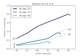
The following figure summarizes these results by taking vertical slices through the survival curves at ages 23, 33 and 43.


In this figure the x-axis is birth cohort and the y-axis is the fraction who have never married.

1) The top line shows that the fraction of women never married by age 23 has increased from 25% for women born in the 40s to 81% for women born in the 90s.

2) The fraction of women unmarried at age 33 has increased from 9% for women born in the 40s to 38% for women born in the 80s, and is projected to be 47% for women born in the 90s.

3) The fraction of women unmarried at age 43 has increased from 8% for women born in the 40s to 17% for women born in the 70s, and is projected to be 36% for women born in the 1990s.

These projections are based on simple assumptions, so we should not treat them as precise predictions, but they are not as naive as a simple straight-line extrapolations of past trends.


Men

The results for men are similar but less extreme.  Here are the estimated survival curves based on a sample of 24652 men in the U.S.  The gray areas show 90% confidence intervals for the estimates due to sampling error.


And projections for the last two cohorts.


Finally, here are the same data plotted with birth cohort on the x-axis.


1) At age 23, the fraction of men who have never married has increased from 66% for men born in the 50s to 88% for men born in the 90s.

2) At age 33, the fraction of unmarried men has increased from 27% to 44%, and is projected to go to 50%.

3) At age 43, the fraction of unmarried men is almost unchanged for men born in the 50s, 60s, and 70s, but is projected to increase to 30% for men born in the 1990s.


Methodology

The NSFG is intended to be representative of the adult U.S. population, but it uses stratified sampling to systematically oversample certain subpopulations, including teenagers and racial minorities.  My analysis takes this design into account (by weighted resampling) to generate results that are representative of the population.

The survival curves are computed by Kaplan-Meier estimation, with confidence intervals computed by resampling.  Missing values are filled by random choice from valid values, so the confidence intervals represent variability due to missing values as well as sampling.

To generate projections, we might consider two factors:

1) If people in the last two cohorts are postponing marriage, we might expect their marriage rates to increase or decrease more slowly.

2) If we extrapolate the trends, we might expect marriage rates to continue to fall or fall faster.

I used an alternative between these extremes: I assume that the hazard function from the previous generation will apply to the next.  This takes into account the possibility of delayed marriage (since there are more unmarried people "at risk" in the projections), but it also assumes a degree of regression to past norms.  In that sense, the projections are probably conservative; that is, they probably underestimate how different the last two cohorts will be from their predecessors.

All the details are in this Jupyter notebook.