Think Complexity: Part Four

My new book, Think Complexity, will be published by O'Reilly Media in March. For people who can't stand to wait that long, I am publishing excerpts here.  If you really can't wait, you can read the free version at thinkcomplex.com.

And we need a blurb.  Think Complexity goes to press soon and we have a space on the back cover for a couple of endorsements.  If you like the book and have something quotable to say about it, let me know.  Thanks!

In Part One I outline the topics in Think Complexity and contrasted a classical physical model of planetary orbits with an example from complexity science: Schelling's model of racial segregation.

In Part Two I outline some of the ways complexity differs from classical science.  In Part Three, I describe differences in the ways complex models are used, and their effects in engineering and (of all things) epistemology.

In this installment, I pull together discussions from two chapters: the Watts-Strogatz model of small world graphs, and the Barabasi-Albert model of scale free networks.  But it all starts with Stanley Milgram.


Stanley Milgram

Stanley Milgram was an American social psychologist who conducted two of the most famous experiments in social science, the Milgram experiment, which studied people's obedience to authority (http://en.wikipedia.org/wiki/Milgram_experiment) and the Small World Experiment (http://en.wikipedia.org/wiki/Small_world_phenomenon), which studied the structure of social networks.

In the Small World Experiment, Milgram sent a package to several randomly-chosen people in Wichita, Kansas, with instructions asking them to forward an enclosed letter to a target person, identified by name and occupation, in Sharon, Massachusetts (which is the town near Boston where I grew up).  The subjects were told that they could mail the letter directly to the target person only if they knew him personally; otherwise they were instructed to send it, and the same instructions, to a relative or friend they thought would be more likely to know the target person.

Many of the letters were never delivered, but of the ones that were it turned out that the average path length---the number of times the letters were forwarded---was about six.  This result was taken to confirm previous observations (and speculations) that the typical distance between any two people in a social network is about ``six degrees of separation.''

This conclusion is surprising because most people expect social networks to be localized---people tend to live near their friends---and in a graph with local connections, path lengths tend to increase in proportion to geographical distance.  For example, most of my friends live nearby, so I would guess that the average distance between nodes in a social network is about 50 miles.  Wichita is about 1600 miles from Boston, so if Milgram's letters traversed typical links in the social network, they should have taken 32 hops, not six.

 Watts and Strogatz

In 1998 Duncan Watts and Steven Strogatz published a paper in  Nature, ``Collective dynamics of 'small-world' networks,'' that proposed an explanation for the small world phenomenon.  You can download it from http://www.nature.com/nature/journal/v393/n6684/abs/393440a0.html.

Watts and Strogatz started with two kinds of graph that were well understood: random graphs and regular graphs.  They looked at two properties of these graphs, clustering and path length.

Clustering is a measure of the ``cliquishness'' of the graph. In a graph, a clique is a subset of nodes that are all connected to each other; in a social network, a clique is a set of friends who all know each other.  Watts and Strogatz defined a clustering coefficient that quantifies the likelihood that two nodes that are connected to the same node are also connected to each other.

Path length is a measure of the average distance between two nodes, which corresponds to the degrees of separation in a social network.

Their initial result is what you might expect: regular graphs have high clustering and high path lengths; random graphs with the same size tend to have low clustering and low path lengths.  So neither of these is a good model of social networks, which seem to combine high clustering with short path lengths.

Their goal was to create a generative model of a social network.  A generative model tries to explain a phenomenon by modeling the process that builds or leads to the phenomenon.  In this case Watts and Strogatz proposed a process for building small-world graphs:

1. Start with a regular graph with n nodes and degree k.  Watts and Strogatz start with a ring lattice, which is a kind of regular graph.  You could replicate their experiment or try instead a graph that is regular but not a ring lattice.
2. Choose a subset of the edges in the graph and ``rewire'' them by replacing them with random edges.  Again, you could replicate the procedure described in the paper or experiment with alternatives.   The proportion of edges that are rewired is a parameter, p, that controls how random the graph is.  With p=0, the graph is regular; with p=1 it is random.

Watts and Strogatz found that small values of p yield graphs with high clustering, like a regular graph, and low path lengths, like a random graph.

 Barabasi and Albert

In 1999 Barabasi and Albert published a paper in Science, ``Emergence of Scaling in Random Networks,'' that characterizes the structure (also called ``topology'') of several real-world networks, including graphs that represent the interconnectivity of movie actors, world-wide web (WWW) pages, and elements in the electrical power grid in the western United States.  You can download the paper from http://www.sciencemag.org/content/286/5439/509.

They measure the degree (number of connections) of each node and compute P(k), the probability that a vertex has degree k; then they plot P(k) versus k on a log-log scale.  The tail of the plot fits a straight line, so they conclude that it obeys a power   law; that is, as k gets large, P(k) is asymptotic to k^(-γ), where γ is a parameter that determines the rate of decay.

They also propose a model that generates random graphs with the same property.  The essential features of the model, which distinguish it from the model and the Watts-Strogatz model, are:

Growth:  Instead of starting with a fixed number of vertices, Barabasi and Albert start with a small graph and add vertices gradually.

Preferential attachment: When a new edge is created, it is more likely to connect to a vertex that already has a large number of edges.  This ``rich get richer'' effect is characteristic of the growth patterns of some real-world networks.

Finally, they show that graphs generated by this model have a distribution of degrees that obeys a power law.  Graphs that have this property are sometimes called scale-free networks; see http://en.wikipedia.org/wiki/Scale-free_network. That name can be confusing because it is the distribution of degrees that is scale-free, not the network.

In order to maximize confusion, distributions that obey a power law are sometimes called scaling distributions because they are invariant under a change of scale.  That means that if you change the units the quantities are expressed in, the slope parameter, γ, doesn't change.  You can read http://en.wikipedia.org/wiki/Power_law for the details, but it is not important for what we are doing here.

 Explanatory models

We started the discussion of networks with Milgram's Small World Experiment, which shows that path lengths in social networks are surprisingly small; hence, ``six degrees of separation''.   When we see something surprising, it is natural to ask ``Why?''  but sometimes it's not clear what kind of answer we are looking for.

One kind of answer is an explanatory model.  The logical structure of an explanatory model is:

1. In a system, S, we see something observable, O, that warrants explanation. 
2. We construct a model, M, that is analogous to the system; that is, there is a correspondence between the elements of the model and the elements of the system.
3. By simulation or mathematical derivation, we show that the model exhibits a behavior, B, that is analogous to O.   
4. We conclude that S exhibits O because S is similar to M, M exhibits B, and B is similar to O.

At its core, this is an argument by analogy, which says that if two things are similar in some ways, they are likely to be similar in other ways.  Argument by analogy can be useful, and explanatory models can be satisfying, but they do not constitute a proof in the mathematical sense of the word.

Remember that all models leave out, or ``abstract away'' details that we think are unimportant.  For any system there are many possible models that include or ignore different features. And there might be models that exhibit different behaviors, B, B' and B'', that are similar to O in different ways. In that case, which model explains O?

The small world phenomenon is an example: the Watts-Strogatz (WS) model and the (BA) model both exhibit small world behavior, but they offer different explanations:

1. The WS model suggests that social networks are ``small'' because they include both strongly-connected clusters and ``weak ties'' that connect clusters.
2. The BA model suggests that social networks are small because they include nodes with high degree that act as hubs, and that   hubs grow, over time, due to preferential attachment. 

As is often the case in young areas of science, the problem is not that we have no explanations, but too many.

Questions

[Think Complexity can be used as a textbook, so it includes exercises and topics for class discussion.  Here are some ideas for discussion and further reading.]

Are these explanations compatible; that is, can they both be right? Which do you find more satisfying as an explanation, and why?  Is there data you could collect, or an experiment you could perform, that would provide evidence in favor of one model over the other?

Choosing among competing models is the topic of Thomas Kuhn's essay, ``Objectivity, Value Judgment, and Theory Choice.''  You can download it here in PDF.  What criteria does Kuhn propose for choosing among competing models? Do these criteria influence your opinion about the WS and BA models? Are there other criteria you think should be considered?

Think Complexity: Part Three

My new book, Think Complexity, will be published by O'Reilly Media in March. For people who can't stand to wait that long, I am publishing excerpts here.  If you really can't wait, you can read the free version at thinkcomplex.com.

In Part One I outline the topics in Think Complexity and contrasted a classical physical model of planetary orbits with an example from complexity science: Schelling's model of racial segregation.

In Part Two I outline some of the ways complexity differs from classical science.  In this installment, I describe differences in the ways complex models are used, and their effects in engineering and (of all things) epistemology.

A new kind of model


Complex models are often appropriate for different purposes and interpretations:

Predictive→explanatory: Schelling's model of segregation might shed light on a complex social phenomenon, but it is not useful for prediction.  On the other hand, a simple model of celestial mechanics can predict solar eclipses, down to the second, years in the future.

Realism→instrumentalism: Classical models lend themselves to a realist interpretation; for example, most people accept that electrons are real things that exist.  Instrumentalism is the view that models can be useful even if the entities they postulate don't exist. George Box wrote what might be the motto of instrumentalism: ``All models are wrong, but some are useful."

Reductionism→holism: Reductionism is the view that the behavior of a system can be explained by understanding its components. For example, the periodic table of the elements is a triumph of reductionism, because it explains the chemical behavior of elements with a simple model of the electrons in an atom.  Holism is the view that some phenomena that appear at the system level do not exist at the level of components, and cannot be explained in component-level terms.

A new kind of engineering

I have been talking about complex systems in the context of science, but complexity is also a cause, and effect, of changes in engineering and the organization of social systems:

Centralized→decentralized: Centralized systems are conceptually simple and easier to analyze, but decentralized systems can be more robust.  For example, in the World Wide Web clients send requests to centralized servers; if the servers are down, the service is unavailable.  In peer-to-peer networks, every node is both a client and a server.  To take down the service, you have to take down every node.

Isolation→interaction: In classical engineering, the complexity of large systems is managed by isolating components and minimizing interactions.  This is still an important engineering principle; nevertheless, the availability of cheap computation makes it increasingly feasible to design systems with complex interactions between components.

One-to-many→many-to-many: In many communication systems, broadcast services are being augmented, and sometimes replaced, by services that allow users to communicate with each other and create, share, and modify content.

Top-down→bottom-up: In social, political and economic systems, many activities that would normally be centrally organized now operate as grassroots movements.  Even armies, which are the canonical example of hierarchical structure, are moving toward devolved command and control.

Analysis→computation: In classical engineering, the space of feasible designs is limited by our capability for analysis.  For example, designing the Eiffel Tower was possible because Gustave Eiffel developed novel analytic techniques, in particular for dealing with wind load.  Now tools for computer-aided design and analysis make it possible to build almost anything that can be imagined.  Frank Gehry's Guggenheim Museum Bilbao is my favorite example.

Design→search: Engineering is sometimes described as a search for solutions in a landscape of possible designs.  Increasingly, the search process can be automated.  For example, genetic algorithms explore large design spaces and discover solutions human engineers would not imagine (or like).  The ultimate genetic algorithm, evolution, notoriously generates designs that violate the rules of human engineering.

A new kind of thinking

We are getting farther afield now, but the shifts I am postulating in the criteria of scientific modeling are related to 20th Century developments in logic and epistemology.

Aristotelian logic→many-valued logic: In traditional logic, any proposition is either true or false. This system lends itself to math-like proofs, but fails (in dramatic ways) for many real-world applications.  Alternatives include many-valued logic, fuzzy logic, and other systems designed to handle indeterminacy, vagueness, and uncertainty.  Bart Kosko discusses some of these systems in Fuzzy Thinking.

Frequentist probability →Bayesianism: Bayesian probability has been around for centuries, but was not widely used until recently, facilitated by the availability of cheap computation and the reluctant acceptance of subjectivity in probabilistic claims.  Sharon Bertsch McGrayne presents this history in The Theory That Would Not Die.

Objective→ subjective: The Enlightenment, and philosophic modernism, are based on belief in objective truth; that is, truths that are independent of the people that hold them.  20th Century developments including quantum mechanics, Godel's Incompleteness Theorem, and Kuhn's study of the history of science called attention to seemingly unavoidable subjectivity in even ``hard sciences'' and mathematics.  Rebecca Goldstein presents the historical context of Godel's proof in Incompleteness.

Physical law→theory→model: Some people distinguish between laws, theories, and models, but I think they are the same thing.  People who use ``law'' are likely to believe that it is objectively true and immutable; people who use ``theory'' concede that it is subject to revision; and ``model'' concedes that it is based on simplification and approximation.

Some concepts that are called ``physical laws'' are really definitions; others are, in effect, the assertion that a model predicts or explains the behavior of a system particularly well. I discuss the nature of physical models later in Think Complexity.

Determinism→indeterminism: Determinism is the view that all events are caused, inevitably, by prior events.  Forms of indeterminism include randomness, probabilistic causation, and fundamental uncertainty. We come back to this topic later in the book.

These trends are not universal or complete, but the center of opinion is shifting along these axes.  As evidence, consider the reaction to Thomas Kuhn's The Structure of Scientific Revolutions, which was reviled when it was published and now considered almost uncontroversial.

These trends are both cause and effect of complexity science.  For example, highly abstracted models are more acceptable now because of the diminished expectation that there should be unique correct model for every system.  Conversely, developments in complex systems challenge determinism and the related concept of physical law.

The excerpts so far have been from Chapter 1 of Think Complexity.  Future excerpts will go into some of these topics in more depth.  In the meantime, you might be interested in this timeline of complexity science (from Wikipedia):

Freshman hordes even more godless!

[This is an update of an article I wrote last year, "Freshman hordes more godless than ever."  There is a followup to this article here.]

For several years I have been following one of the most under-reported stories of the decade: the fraction of college freshmen who report no religious preference has more than tripled since 1985, from 8% to 25%, and the trend is accelerating.

Similarly, students reporting that in the last year they have never attended a religious service has grown from 8% to more than 27%.

My analysis is based on survey results from the Cooperative Institutional Research Program (CIRP) of the Higher Education Research Insitute (HERI).  In 2011, more than 200,000 students at 270 colleges and universities completed the CIRP Freshman Survey, which includes questions about students’ backgrounds, activities, and attitudes.


In one question, students select their “current religious preference,” from a choice of seventeen common religions, “Other religion,” or “None.”


Another question asks students how often they “attended a religious service” in the last year. The choices are “Frequently,” “Occasionally,” and “Not at all.” Students are instructed to select “Occasionally” if they attended one or more times.

This figure shows students' responses over the history of the survey:

It's clear that both measurements are increasing, and it looks like they might be accelerating.  To make that more precise, I fit a parabola to each curve.  This figure shows the data for "No religion" and a least squares fit:

The red line shows the fitted model; the dark gray area shows the sample error of the model.  The lighter gray area shows the sum of the sampling error and the residual error.  R² for this model is 0.95; the p-values for the model and the parameters are < 0.001. 


Similarly, here is the data for "No attendance" and a least squares fit:

R² for this model is 0.89, and again the p-values are effectively 0. [Note for stats geeks: as it happens, the coefficient of the linear term is close to zero, so it is not statistically significant.  My first thought was to remove it from the model, but if I did that, I would understate the sampling error of the model.  In this case, it is correct to keep an "insignificant" variable in the model; the fact that it is near zero doesn't mean we can ignore it, or the error associated with it.]


To test more explicitly whether the growth is accelerating, I computed the change from one year to the next in percentage points.  The following figure shows these changes and a least squares fit:

Subtraction amplifies noise, so for this model R² is only 0.24, but the p-value of the slope is 0.002, so this data provides strong evidence of acceleration.  The slope is 0.035 percentage points per year.


Based on this model, the predicted change for next year is 1 percentage point, so we expect the fraction of freshmen reporting no religious preference to be 26%.


The gender gap


Since the beginning of the CIRP survey, more men than women have reported no religious preference:

And the gender gap seems to be growing.  Here is the difference between men and women, in percentage points, and a least squares fit:

R² for this model is 0.44; the slope is 0.035 percentage points per year, with p-value < 0.0001.

Discussion



I first wrote about this in 2007, in this article for Free Inquiry magazine.  There I wrote:

College students are hardly a random sample of the population. People with more education are less likely to believe in heaven, the devil, miracles, and the literal truth of the Christian Bible. However, contrary to many people’s expectations, educated people are more likely to attend services. So, we expect the students in this sample to be less believing than the general population but also more observant. 

There is reason to think that the rate of secularization in the general population is faster than what we see in this sample. Over the lifetime of the CIRP survey, college education has democratized; the percentage of high-school graduates who enter college immediately after graduation has increased from roughly 50 percent in 1970 to 65 percent in 2003. Over this time, CIRP has included more poor students, more racial minorities, and more students from families with less education. These groups tend to be more religious than the general population, so we expect their participation to increase the religiosity in the sample. Thus, the observed decrease probably underestimates the trend in the general population. 

The theory of secularization—that there is a global, long-term trend away from religion—is controversial. Early sociologists, notably Max Weber, hypothesized that secularization is a predictable effect of rationalization—the increasing tendency for social actions to be based on reason rather than emotion or tradition.

In the 1950s and 1960s, many sociologists of religion defended strong theories of secularization, but, since then, several of them—including Peter Berger and Harvey Cox—have reversed their positions, arguing that religion is resurging in some areas, including the United States. 

The data presented here speak directly to this debate. The CIRP survey has posed almost the same questions to a large sample of a consistently defined group for almost forty years, and the results show a clear and consistent trend away from both identification with religious sects and participation in religious services. These data make a strong case for secularization in the United States that has, if anything, accelerated in the last decade.

Data Source

Data from the 2011 CIRP Survey are reported in The American Freshman: National Norms for Fall 2011, Pryor, J. H., DeAngelo, L., Palucki Blake, L., Hurtado, S., & Tran, S., Jan 2012.


This and all previous reports are available from the HERI publications page.

Think Complexity, Part Two

My new book, Think Complexity, will be published by O'Reilly Media in March. For people who can't stand to wait that long, I am publishing excerpts here.  If you really can't wait, you can read the free version at thinkcomplex.com.

In the previous installment I outlined the topics in Think Complexity and contrasted a classical physical model of planetary orbits with an example from complexity science: Schelling's model of racial segregation.  In this installment I outline some of the ways complexity differs from classical science.

Paradigm shift?  

When I describe this book to people, I am often asked if this new kind of science is a paradigm shift.  I don't think so, and here's why.   Thomas Kuhn introduced the term ``paradigm shift'' in The Structure of Scientific Revolutions in 1962.  It refers to a process in the history of science where the basic assumptions of a field change, or where one theory is replaced by another. He presents as examples the Copernican revolution, the displacement of phlogiston by the oxygen model of combustion, and the emergence of relativity.

The development of complexity science is not the replacement of an older model, but (in my opinion) a gradual shift in the criteria models are judged by, and in the kinds of models that are considered acceptable.  For example, classical models tend to be law-based, expressed in the form of equations, and solved by mathematical derivation.  Models that fall under the umbrella of complexity are often rule-based, expressed as computations, and simulated rather than analyzed.  Not everyone finds these models satisfactory.

For example, in Sync, Steven Strogatz writes about his model of spontaneous synchronization in some species of fireflies.  He presents a simulation that demonstrates the phenomenon, but then writes:

I repeated the simulation dozens of times, for other random initial conditions and for other numbers of oscillators.  Sync every time. [...] The challenge now was to prove it.  Only an ironclad proof would demonstrate, in a way that no computer ever could, that sync was inevitable; and the best kind of proof would clarify why it was inevitable.  

Strogatz is a mathematician, so his enthusiasm for proofs is understandable, but his proof doesn't address what is, to me, the most interesting part the phenomenon.  In order to prove that ``sync was inevitable,'' Strogatz makes several simplifying assumptions, in particular that each firefly can see all the others.

In my opinion, it is more interesting to explain how an entire valley of fireflies can synchronize despite the fact that they cannot all see each other.  Think Complexity discusses how this kind of global behavior emerges from local interactions. Explanations of these phenomena often use agent-based models, which explore (in ways that would be difficult or impossible with mathematical analysis) the conditions that allow or prevent synchronization.

I am a computer scientist, so my enthusiasm for computational models is probably no surprise.  I don't mean to say that Strogatz is wrong, but rather that people disagree about what questions to ask and what tools to use to answer them.  These decisions are based on value judgments, so there is no reason to expect agreement.  Nevertheless, there is rough consensus among scientists about which models are considered good science, and which others are fringe science, pseudoscience, or not science at all.

I claim, and this is a central thesis of the book, that the criteria this consensus is based on change over time, and that the emergence of complexity science reflects a gradual shift in these criteria.

The axes of scientific models

I have described classical models as based on physical laws, expressed in the form of equations, and solved by mathematical analysis; conversely, models of complexity systems are often based on simple rules and implemented as computations.  We can think of this trend as a shift over time along two axes:

Equation-based→ simulation-based
Analysis→computation

The new kind of science is different in several other ways:

Continuous→discrete: Classical models tend to be based on continuous mathematics, like calculus; models of complex systems are often based on discrete mathematics, including graphs and cellular automata.

Linear→non-linear: Classical models are often linear, or use linear approximations to non-linear systems; complexity science is more friendly to non-linear models.  One example is chaos theory, which explores the dynamics of systems of non-linear equations.

Deterministic→stochastic: Classical models are usually deterministic, which may reflect underlying philosophical determinism; complex models often feature randomness.

Abstract→detailed: In classical models, planets are point masses, planes are frictionless, and cows are spherical (see http://en.wikipedia.org/wiki/Spherical_cow).  Simplifications like these are often necessary for analysis, but computational models can be more realistic.

One, two→many: In celestial mechanics, the two-body problem can be solved analytically; the three-body problem cannot.  Where classical models are often limited to small numbers of interacting elements, complexity science works with larger complexes (which is where the name comes from).

Homogeneous→composite: In classical models, the elements tend to be interchangeable; complex models more often include heterogeneity.

These are generalizations, so we should not take them too seriously. And I don't mean to deprecate classical science.  A more complicated model is not necessarily better; in fact, it is usually worse.

Also, I don't mean to say that these changes are abrupt or complete. Rather, there is a gradual migration in the frontier of what is considered acceptable, respectable work.  Some tools that used to be regarded with suspicion are now common, and some  models that were widely accepted are now regarded with scrutiny.  For example, when Appel and Haken proved the four-color theorem in 1976, they used a computer to enumerate 1,936 special cases that were, in some sense, lemmas of their proof.  At the time, many mathematicians did not consider the theorem truly proved.  Now computer-assisted proofs are common and generally (but not universally) accepted.

Conversely, a substantial body of economic analysis is based on a model of human behavior called ``Economic man,'' or, with tongue in cheek, Homo economicus.  Research based on this model was highly-regarded for several decades, especially if it involved mathematical virtuosity.  More recently, this model is treated with more skepticism, and models that include imperfect information and bounded rationality are hot topics.

At this point I have laid out a lot of ideas for one article, and explained them very briefly.  Think Complexity gets into these topics in more detail, but I will stop here for now.  Next time I will talk about related shifts in engineering and (a little farther afield) in ways of thinking.

Think Complexity

Think Complexity

On Friday I turned in the manuscript for Think Complexity, which will be published by O'Reilly Media in March (or, at least, that's the schedule). For people who can't stand to wait that long, I am going to publish excerpts here.  And if you really can't wait, you can read the free version at thinkcomplex.com.

The book is about data structures and algorithms, intermediate programming in Python, computational modeling and the philosophy of science:

• Data structures and algorithms: A data structure is a collection of data elements organized in a way that supports particular operations.  For example, a Python dictionary organizes key-value pairs in a way that provides fast mapping from keys to values, but mapping from values to keys is slower. An algorithm is a mechanical process for performing a computation. Designing efficient programs often involves the co-evolution of data structures and the algorithms that use them.  For example, in the first few chapters I present graphs, data structures that implement graphs, and graph algorithms based on those data structures.
• Python programming: Think Complexity picks up where Think Python leaves off.  I assume that you have read that book or have equivalent knowledge of Python.  I try to emphasize fundamental ideas that apply to programming in many languages, but along the way I present some useful features that are specific to Python.
• Computational modeling: A model is a simplified description of a system used for simulation or analysis. Computational models are designed to take advantage of cheap, fast computation.
• Philosophy of science: The experiments and results in this book raise questions relevant to the philosophy of science, including the nature of scientific laws, theory choice, realism and instrumentalism, holism and reductionism, and epistemology.

The book is also about complexity science, which is an interdisciplinary field---at the intersection of mathematics, computer science and natural science---that focuses on discrete models of physical systems.  In particular, it focuses on complex systems, which are systems with many interacting components.

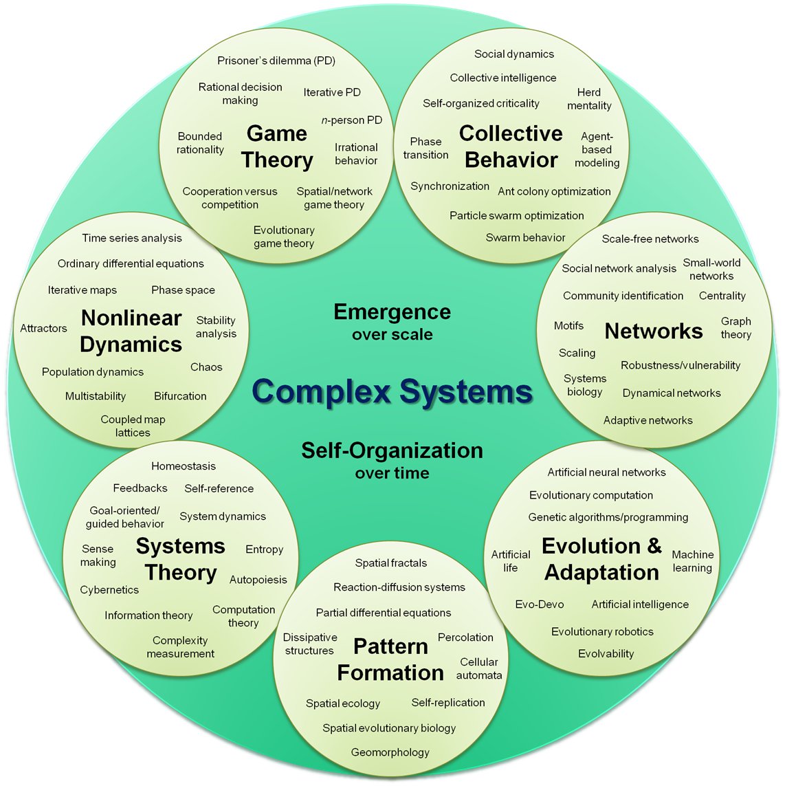
Complex systems include networks and graphs, cellular automata, agent-based models and swarms, fractals and self-organizing systems, chaotic systems and cybernetic systems.  Here is a framework for these topics (from http://en.wikipedia.org/wiki/Complex_systems).

A new kind of science?

In 2002 Stephen Wolfram published A New Kind of Science where he presents his and others' work on cellular automata and describes a scientific approach to the study of computational systems.  There's a chapter about cellular automata in the book, but for now I'm going to borrow his title for something a little broader.

I think complexity is a ``new kind of science'' not because it applies the tools of science to a new subject, but because it uses different tools, allows different kinds of work, and ultimately changes what we mean by ``science.''

To demonstrate the difference, I'll start with an example of classical science: suppose someone asked you why planetary orbits are elliptical.  You might invoke Newton's law of universal gravitation and use it to write a differential equation that describes planetary motion.  Then you could solve the differential equation and show that the solution is an ellipse.  Voila!

Most people find this kind of explanation satisfying.  It includes a mathematical derivation---so it has some of the rigor of a proof---and it explains a specific observation, elliptical orbits, by appealing to a general principle, gravitation.

Let me contrast that with a different kind of explanation.  Suppose you move to a city like Detroit that is racially segregated, and you want to know why it's like that.  If you do some research, you might find a paper by Thomas Schelling called ``Dynamic Models of Segregation,'' which proposes a simple model of racial segregation (you can download the paper here).

Here is an outline of the paper's primary experiment:

• The Schelling model of the city is an array of cells where each cell represents a house.  The houses are occupied by two kinds of agents, labeled red and blue, in roughly equal numbers.  About 10% of the houses are empty.   
• At any point in time, an agent might be happy or unhappy, depending on the other agents in the neighborhood.  In one version of the model, agents are happy if they have at least two neighbors like themselves, and unhappy if they have one or zero.
• The simulation proceeds by choosing an agent at random and checking to see whether it is happy.  If so, nothing happens; if not, the agent chooses one of the unoccupied cells at random and moves.

If you start with a simulated city that is entirely unsegregated and run the model for a short time, clusters of similar agents appear.  As time passes, the clusters grow and coalesce until there are a small number of large clusters and most agents live in homogeneous neighborhoods.

The degree of segregation in the model is surprising, and it suggests an explanation of segregation in real cities.  Maybe Detroit is segregated because people prefer not to be greatly outnumbered and will move if the composition of their neighborhoods makes them unhappy.    

Is this explanation satisfying in the same way as the explanation of planetary motion?  Most people would say not, but why?

Most obviously, the Schelling model is highly abstract, which is to say not realistic.  It is tempting to say that people are more complex than planets, but when you think about it, planets are just as complex as people (especially the ones that have people).

Both systems are complex, and both models are based on simplifications; for example, in the model of planetary motion we include forces between the planet and its sun, and ignore interactions between planets.

The important difference is that, for planetary motion, we can defend the model by showing that the forces we ignore are smaller than the ones we include.  And we can extend the model to include other interactions and show that the effect is small.  For Schelling's model it is harder to justify the simplifications.

To make matters worse, Schelling's model doesn't appeal to any physical laws, and it uses only simple computation, not mathematical derivation.  Models like Schelling's don't look like classical science, and many people find them less compelling, at least at first. But as I will try to demonstrate, these models do useful work, including prediction, explanation, and design.  One of the goals of Think Complexity is to explain how.

In the next excerpt, I will present some of the ways I think complexity science differs from classical science.  But in the meantime I welcome comments on Part One.

Some of my best friends are crackpots

I have a soft spot for crank science.  Recently I visited Norumbega Tower, which is an enduring monument to the crackpot theories of Eben Norton Horsford, inventor of double-acting baking powder and faux history.  But that's not what this article is about.

This article is about the Variability Hypothesis, which (quoth Wikipedia):

"originated in the early nineteenth century with Johann Meckel, who argued that males have a greater range of ability than females, especially in intelligence. In other words, he believed that most geniuses and most mentally retarded people are men. Because he considered males to be the 'superior animal,' Meckel concluded that females' lack of variation was a sign of inferiority."

I particularly like the last part, because I suspect that if it turns out that women are actually more variable, Meckel would take that as a sign of inferiority, too.  Anyway, you will not be surprised to hear that evidence for the Variability Hypothesis is mixed at best.

Nevertheless, it came up in my class recently when we looked at data from the CDC's Behavioral Risk Factor Surveillance System (BRFSS), specifically the self-reported height of adult American men and women.  The dataset includes responses from 154407 men and 254722 women.  Here's what we found:

• The average height for men is 178 cm; the average height for women is 163 cm.  So men are taller, on average.  No surprises so far.
• For men the standard deviation is 7.7 cm; for women is it 7.3 cm.  So in absolute terms, men's heights are more variable.
• But to compare variability between groups, it is more meaningful to use the coefficient of variation (CV), which is the standard deviation divided by the mean.  It is a dimensionless measure of variability relative to scale.  For men CV is 0.0433; for women it is 0.0444.

That's very close, so we could conclude that this dataset provides no support for the Variability Hypothesis.  But in keeping with the theme of this blog, I won't be happy until I have overthought the question.  And along the way I want to use this problem to demonstrate Bayesian estimation in 2 dimensions.

 Bayesian estimation in 2-D

In previous articles I have presented Bayesian estimation for the number of species in a biological sample and the age of a renal tumor.  But those are both 1-D problems.  Estimating the mean and variance of a sample is a 2-D problem.  There are analytic solutions for several forms of the prior distribution, but as usual I will demonstrate a computational approach.

I'll present the code for the update first, and get back to the prior.  Here's what the update looks like:


def LogUpdate(suite, evidence):
    for hypo in suite.Values():
        likelihood = LogLikelihood(evidence, hypo)
        suite.Incr(hypo, likelihood)

suite is a Pmf object that maps from each hypothesis to its probability.  While we're performing the update, the probabilities are unnormalized, which is why they are called likelihoods.  And the whole thing happens under a log transform, because otherwise the likelihoods get so small they get rounded off to zero (see underflow).

Here's the function that computes likelihoods:


def LogLikelihood(evidence, hypo):
    t = evidence
    mu, sigma = hypo


    total = Summation(t, mu)
    return -len(t) * math.log(sigma) - total / 2 / sigma**2

evidence is the tuple of heights in centimeters; hypo is a tuple of hypothetical values for mu and sigma.  Summation computes the sum of the squared deviations from mu; the return value is the log likelihood of getting this sample from a Gaussian distribution with the hypothetical parameters.

I pulled Summation out into a separate function because it gets called repeatedly with the same parameters, so I can improve the run time (a lot) by caching previous results:


def Summation(t, mu, cache={}):
    try:
        return cache[t, mu]
    except KeyError:
        total = sum((x-mu)**2 for x in t)
        cache[t, mu] = total
        return total

That's it for the update.  Now we need a prior.  One option is a uniform prior where mu can be any value and sigma can be any positive value.  In practice, there is no point in evaluating values far from the true parameters, because their likelihoods will be vanishingly small.  So we'll use the data to choose the range for the prior, then use the data to update the prior.

That might sound completely bogus, because we are using the same data twice.  But choosing the range for the prior is just a computational convenience; it has no effect on the result, as long as the range is wide enough that the likelihood for values outside the range is effectively zero.

To choose the prior range for mu and sigma, I use the conventional estimators and their standard errors.  Here's the code:


def MakeUniformPrior(t, num_points, label, spread=3.0):
    
    # estimate mean and stddev of t
    n = len(t)
    xbar, S2 = thinkstats.MeanVar(t)
    sighat = math.sqrt(S2)


    # compute standard error for mu and the range of ms
    stderr_xbar = sighat / math.sqrt(n)
    mspread = spread * stderr_xbar
    ms = numpy.linspace(xbar-mspread, xbar+mspread, num_points)


    # compute standard error for sigma and the range of ss
    stderr_sighat = sighat / math.sqrt(2 * (n-1))
    sspread = spread * stderr_sighat
    ss = numpy.linspace(sighat-sspread, sighat+sspread, num_points)


    # populate the PMF
    pmf = Pmf.Pmf(name=label)
    for m in ms:
        for s in ss:
            pmf.Set((m, s), 1)
    return ms, ss, pmf

Finally, here's the code that makes the prior, updates it, and normalizes the posterior:

def EstimateParameters(t, label, num_points=31):

    xs, ys, suite = MakeUniformPrior(t, num_points, label)

    suite.Log()

    LogUpdate(suite, tuple(t))

    suite.Exp()

    suite.Normalize()

    return xs, ys, suite

Ok, that was more code than I usually put in these articles.  You can download it all from thinkcomplex.com/bayes_height.py.

Results

The result is a map from pairs of mu and sigma to probabilities; one simple way to display the map is a contour plot.  Here is the result for men:

And for women:

As expected, the central location is near the estimated parameters.  But with this result in numerical form is that it is easy to compute the marginal distributions for mu and sigma, or their confidence intervals.  We can also compute posterior distributions for CV, and compare the distributions CV for men and women:

Since there is no overlap between the distributions, we can conclude that the small observed difference is statistically significant; or, if we want to be more Bayesian about it, we can compute the probability that the CV for women is higher, which is pretty close to 1.

Finally we conclude:

• The standard deviation of height for men is higher.
• But the coefficient of variation is slightly lower.
• Even though the difference is tiny, it is very unlikely to be due to chance.
• And therefore women are inferior.

Hey, I told you I have a soft spot for crank science.

Frank is a scoundrel, probably

My friend Ted Bunn wrote an article, "Who knows what evil lurks in the hearts of men? The Bayesian doesn’t care," inspired in part by one of my posts, "Repeated tests: how bad can it be?"

He presents this scenario:

Frank and Betsy are wondering whether a particular coin is a fair coin (i.e., comes up heads and tails equally often when flipped).  Frank, being a go-getter type, offers to do some tests to find out. He takes the coin away, flips it a bunch of times, and eventually comes back to Betsy to report his results. 

“I flipped the coin 3022 times,” he says, “and it came up heads 1583 times. That’s 72 more heads than you’d expect with a fair coin. I worked out the p-value — that is, the probability of this large an excess occurring if the coin is fair — and it’s under 1%. So we can conclude that the coin is unfair at a significance level of  1% (or ’99% confidence’ as physicists often say).”

And suggests that there are two ways Betsy can interpret this report (again, quoting Ted):

1. Frank is an honest man, who has followed completely orthodox (frequentist) statistical procedure. To be specific, he decided on the exact protocol for his test (including, for some reason, the decision to do 3022 trials) in advance.
2. Frank is a scoundrel who, for some reason, wants to reach the conclusion that the coin is unfair. He comes up with a nefarious plan: he keeps flipping the coin for as long as it takes to reach that 1% significance threshold, and then he stops and reports his results.

Finally, Ted asks, "What should Betsy conclude on the basis of the information Frank has given her?"  If you want to know Ted's answer, you have to read his article (and you should -- it is very interesting).

But I'm going to give you my answer: Frank is a scoundrel.  Well, probably.

I'll follow Ted by making one more assumption: "Suppose that Betsy’s initial belief is that 95% of coins are fair — that is, the probability P that they come up heads is exactly 0.5."  Now we can evaluate the evidence that Frank is a scoundrel.

If Frank is a scoundrel, the probability that he reports a positive result is 1, provided that he is willing to keep flipping long enough, or 1-x, for small x, if we put a bound on the number of flips he is willing to do.  So

P(positive test | Frank is a scoundrel) = 1-x

If Frank is honest, then the probability of a positive result is

P(fair coin) P(false positive | fair coin) + P(biased coin) * P(true positive | biased coin)

Betsy believes that P(fair coin) is 95% and P(biased coin) is 5%.  Since Frank's significance level is 1%, P(false positive | fair coin) is 1%.

The probability of a true positive is the power of the test, which depends on how biased the coin actually is.  But I will make the approximation that 3022 flips is enough to detect any substantial bias, so I'll take P(true positive | biased coin) = 1-y, for small y.  So,

P(positive test | Frank is honest) = (0.95)(0.01) + (0.05)(1-y)

As x and y get small, the likelihood ratio is (1 / 0.0595), which is about 17.  So that is fairly strong evidence that Frank is a scoundrel.

I don't know about Betsy's prior beliefs about Frank, so you will have to fill in your own punchline about her posterior.