In most foot races, everyone starts at the same time. If you are a fast runner, you usually pass a lot of people at the beginning of the race, but after a few miles everyone around you is going at the same speed.
Last September I ran the Reach the Beach relay, where teams of 12 run 209 miles in New Hampshire from Cannon to Hampton Beach. While I was running my second leg, I noticed an odd phenomenon: when I overtook another runner, I was usually much faster, and when other runners overtook me, they were usually much faster.
At first I thought that the distribution of speeds might be bimodal; that is, there were many slow runners and many fast runners, but few at my speed. Then I realized that I was the victim of selection bias.
The race was unusual in two ways: it used a staggered start, so teams started at different times; also, many teams included runners at different levels of ability. As a result, runners were spread out along the course with little relationship between speed and location. When I started my leg, the runners near me were (pretty much) a random sample of the runners in the race.
So where does the bias come from? During my time on the course, the chance of overtaking a runner, or being overtaken, is proportional to the difference in our speeds. To see why, think about the extremes. If another runner is going at the same speed as me, neither of us will overtake the other. If someone is going so fast that they cover the entire course while I am running, they are certain to overtake me.
To see what effect this has on the distribution of speeds, I downloaded the results from a race I ran last spring (the James Joyce Ramble 10K in Dedham MA) and converted the pace of each runner to MPH. Here’s what the probability mass function (PMF) of speeds looks like in a normal road race (not a relay):
It is bell-shaped, which suggests a Gaussian distribution. There are more fast runners than we would expect in a Gaussian distribution, but that’s a topic for another post.
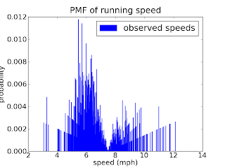
Now, let’s see what this looks like from the point of view of a runner in a relay race going 7.5 MPH. For each speed, x, I apply a weight proportional to abs(x-7.5). The result looks like this:
It’s bimodal, with many runners faster and slower than the observer, but few runners at or near the same speed. So that’s consistent with my observation while I was running. (The tails are spiky, but that’s an artifact of the small sample size. I could apply some smoothing, but I like to keep data-mangling to a minimum.)
One of the nice things about long-distance running is that you have time to think about things like this.
-----
Appendix: Here’s the code I used to compute the observed speeds:
def BiasPmf(pmf, speed, name=None):
"""Returns a new PDF representing speeds observed at a given speed.
The chance of observing a runner is proportional to the difference in speed.
Args:
pmf: distribution of actual speeds
speed: speed of the observing runner
name: string name for the new dist
Returns:
Pmf object
"""
new = pmf.Copy(name=name)
for val, prob in new.Items():
diff = abs(val - speed)
new.Mult(val, diff)
new.Normalize()
return new
This code uses the PMF library, which you can read about in my book, Think Stats.


No comments:
Post a Comment