Thursday, August 27, 2015

Bayes theorem in real life

I had a chance to practice Bayesian inference in real life today: at 1pm my wife called to tell me that the carbon monoxide (CO) alarm at the house was going off.  Immediately two hypotheses came to mind: (1) there is a dangerous amount of CO in my house, (2) it's a false alarm.

It's summer and all the windows are open in the house.  The furnace is not running and we don't have a gas stove.  And the detector is about 10 years old.  This background information makes a false alarm more plausible, so I started with a low prior for (1).  Since my wife was on her way out anyway, I suggested she disconnect the detector, turn on a fan, and leave.

After we hung up, I searched for information on CO detectors and false alarms.  Apparently, the rate of false alarms is low, at least in once sense: CO detectors are very specific, that is, unlikely to go off because of anything other than CO.  Of course the other possibility is that the detector is broken.  On balance, this information made me less confident of a false alarm.

I tried to think of other possibilities:
  • A major street nearby is being paved.  Does fresh pavement off-gas anything that would set off a CO detector?
  • At a construction site down the street, they just poured a concrete foundation, and my neighbor is having some masonry done.  Does fresh concrete off-gas CO?  I vaguely remember that it sequesters oxygen, which turned out to be a problem for one of the Biosphere projects.
  • What about a smoldering fire inside a wall?  Could it produce enough CO to set off the detector, but not enough smoke to set off the smoke alarms?
The first two seemed unlikely, but the third seemed plausible.  In fact, it seemed plausible enough that I decided to go home and check it out.  When I got there, the windows were open and fans were running, so I figured the air had exchanged at least once, and the detector had a chance to reset.

I put on over-the-head 30dB earmuffs and plugged the detector back in.  It went off immediately.  I plugged it into an outlet in another room, and it went off immediately.  At this point it seemed unlikely that every room in my wide-open, highly ventilated house was full of CO.

I still couldn't rule out a smoldering fire, but it sure seemed unlikely.  Nevertheless, I called the fire department, using their non-emergency number to preserve some dignity, and told them the story.  They sent a truck, walked through the house with a gas detector, and reported no CO anywhere.

One of the fireman told me that CO detectors are good for about 7 years, so it's time for a new one.  And while I'm at it, he suggested, I should get one more for the first floor (currently I have one in the basement and one on the second floor).  And that's what I did.

So what have we learned?

1) Make sure you have a CO detector on each floor of your house.  CO poisoning is no joke.  Want proof?  Run this search query any time.  Chances are you'll find several serious accidents within the last week or so.

2)  Replace detectors after 5-7 years.  Apparently newer ones have an end-of-life alert, so you don't have to keep track.  If you have an older one, figure out the replacement day and put it on your calendar.

3) Think like a Bayesian.  As you get more information, update your probabilities, and change your decisions accordingly.  My initial estimate for the probability of false alarm was so high, I decided not to check it out.  As I thought of more possible explanations, the probability of a real problem crept higher.  It was still very low, but high enough that I decided to go home.

4) On the other hand, a strictly Bayesian framework doesn't always fit real-world thinking.  In this case, my decision flipped when I thought of a new hypothesis (a smoldering fire).  Should I consider that a new piece of information and update my prior?  Or is it a new piece of background information that caused me to go back, revise my prior, and start over?  In practice, it makes no difference.  But from a Bayesian point of view, it's not quite as neat as it might be.


Tuesday, August 18, 2015

The Inspection Paradox is Everywhere


I have updated this article with new data, better code, and friendlier data visualization. 
You can read the new version here.

 
The Inspection Paradox is Everywhere


The inspection paradox is a common source of confusion, an occasional source of error, and an opportunity for clever experimental design.  Most people are unaware of it, but like the cue marks that appear in movies to signal reel changes, once you notice it, you can’t stop seeing it.


A common example is the apparent paradox of class sizes.  Suppose you ask college students how big their classes are and average the responses.  The result might be 56.  But if you ask the school for the average class size, they might say 31.  It sounds like someone is lying, but they could both be right.

The problem is that when you survey students, you oversample large classes.  If there are 10 students in a class, you have 10 chances to sample that class.  If there are 100 students, you have 100 chances.  In general, if the class size is x, it will be overrepresented in the sample by a factor of x.


That’s not necessarily a mistake.  If you want to quantify student experience, the average across students might be a more meaningful statistic than the average across classes.  But you have to be clear about what you are measuring and how you report it.


By the way, I didn’t make up the numbers in this example.  They come from class sizes reported by Purdue University for undergraduate classes in the 2013-14 academic year.  https://www.purdue.edu/datadigest/2013-14/InstrStuLIfe/DistUGClasses.html


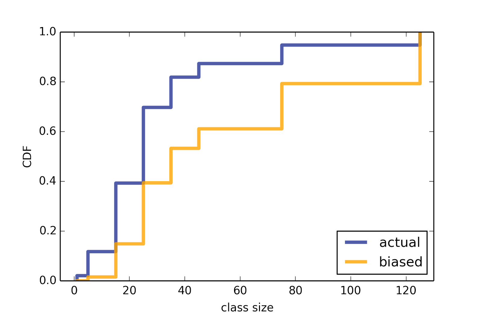
From the data in their report, I estimate the actual distribution of class sizes; then I compute the “biased” distribution you would get by sampling students.  The CDFs of these distributions are in Figure 1.


Going the other way, if you are given the biased distribution, you can invert the process to estimate the actual distribution.  You could use this strategy if the actual distribution is not available, or if it is easier to run the biased sampling process.


purdue3.png
Figure 1: Undergraduate class sizes at Purdue University, 2013-14 academic year: actual distribution and biased view as seen by students.


The same effect applies to passenger planes.  Airlines complain that they are losing money because so many flights are nearly empty.  At the same time passengers complain that flying is miserable because planes are too full.  They could both be right.  When a flight is nearly empty, only a few passengers enjoy the extra space.  But when a flight is full, many passengers feel the crunch.


Once you notice the inspection paradox, you see it everywhere.  Does it seem like you can never get a taxi when you need one?  Part of the problem is that when there is a surplus of taxis, only a few customers enjoy it.  When there is a shortage, many people feel the pain.


Another example happens when you are waiting for public transportation.  Buses and trains are supposed to arrive at constant intervals, but in practice some intervals are longer than others.  With your luck, you might think you are more likely to arrive during a long interval.  It turns out you are right: a random arrival is more likely to fall in a long interval because, well, it’s longer.


To quantify this effect, I collected data from the Red Line in Boston.  Using their real-time data service, I recorded the arrival times for 70 trains between 4pm and 5pm over several days.
redline2.png
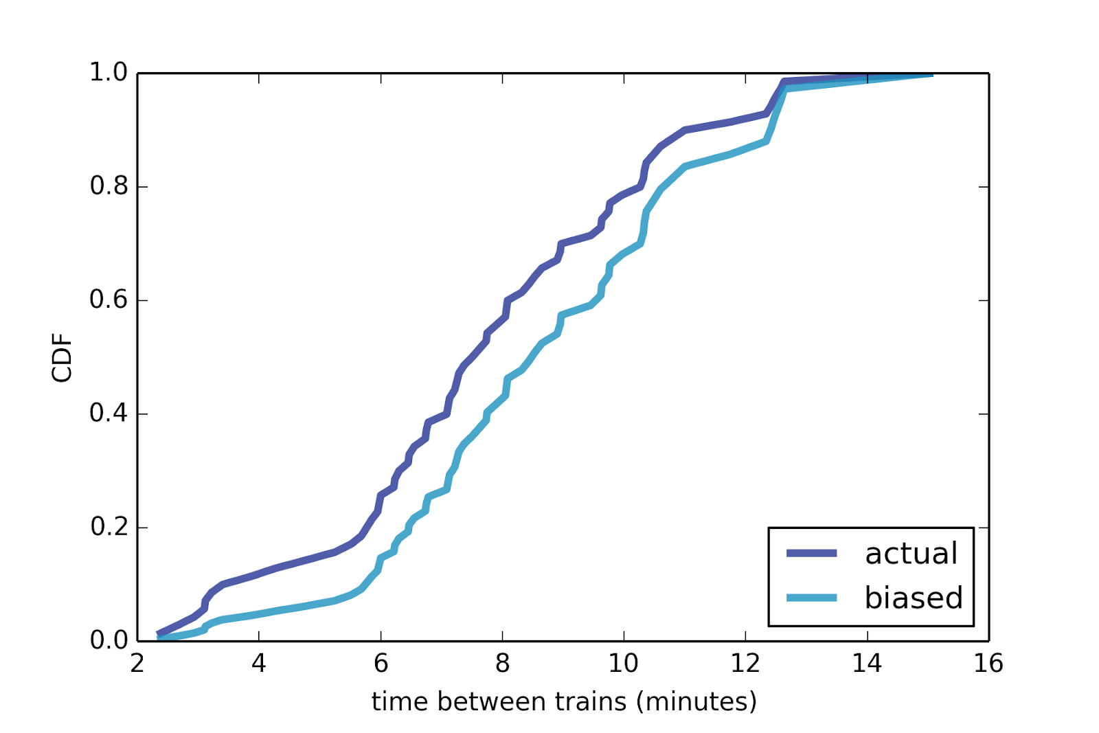
Figure 2: Distribution of time between trains on the Red Line in Boston, between 4pm and 5pm.


The shortest gap between trains was less than 3 minutes; the longest was more than 15.  Figure 2 shows the actual distribution of time between trains, and the biased distribution that would be observed by passengers.  The average time between trains is 7.8 minutes, so we might expect the average wait time to be 3.8 minutes.  But the average of the biased distribution is 8.8 minutes, and the average wait time for passengers is 4.4 minutes, about 15% longer.


In this case the difference between the two distributions is not very big because the variance of the actual distribution is moderate.  When the actual distribution is long-tailed, the effect of the inspection paradox can be much bigger.


An example of a long-tailed distribution comes up in the context of social networks.  In 1991, Scott Feld presented the “friendship paradox”: the observation that most people have fewer friends than their friends have.  He studied real-life friends, but the same effect appears in online networks: if you choose a random Facebook user, and then choose one of their friends at random, the chance is about 80% that the friend has more friends.


The friendship paradox is a form of the inspection paradox.  When you choose a random user, every user is equally likely.  But when you choose one of their friends, you are more likely to choose someone with a lot of friends.  Specifically, someone with x friends is overrepresented by a factor of x.


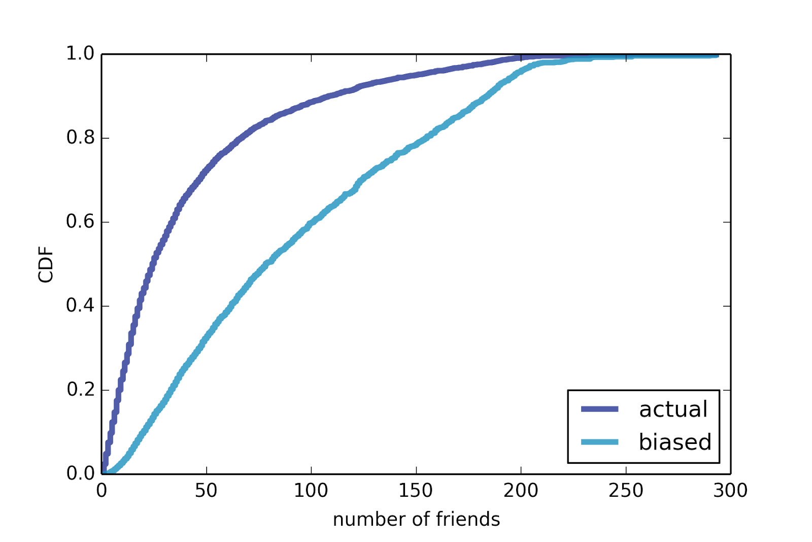
To demonstrate the effect, I use data from the Stanford Large Network Dataset Collection (http://snap.stanford.edu/data), which includes a sample of about 4000 Facebook users.  We can compute the number of friends each user has and plot the distribution, shown in Figure 3.  The distribution is skewed: most users have only a few friends, but some have hundreds.

We can also compute the biased distribution we would get by choosing choosing random friends, also shown in Figure 3.  The difference  is huge.  In this dataset, the average user has 42 friends; the average friend has more than twice as many, 91.
social4.png
Figure 3: Number of online friends for Facebook users: actual distribution and biased distribution seen by sampling friends.


Some examples of the inspection paradox are more subtle.  One of them occurred to me when I ran a 209-mile relay race in New Hampshire.  I ran the sixth leg for my team, so when I started running, I jumped into the middle of the race.  After a few miles I noticed something unusual: when I overtook slower runners, they were usually much slower; and when faster runners passed me, they were usually much faster.


At first I thought the distribution of runners was bimodal, with many slow runners, many fast runners, and few runners like me in the middle.  Then I realized that I was fooled by the inspection paradox.


In many long relay races, teams start at different times, and most teams include a mix of faster and slower runners.  As a result, runners at different speeds end up spread over the course; if you stand at  random spot and watch runners go by, you see a nearly representative sample of speeds.  But if you jump into the race in the middle, the sample you see depends on your speed.


Whatever speed you run, you are more likely to pass very slow runners, more likely to be overtaken by fast runners, and unlikely to see anyone running at the same speed as you.  The chance of seeing another runner is proportional to the difference between your speed and theirs.


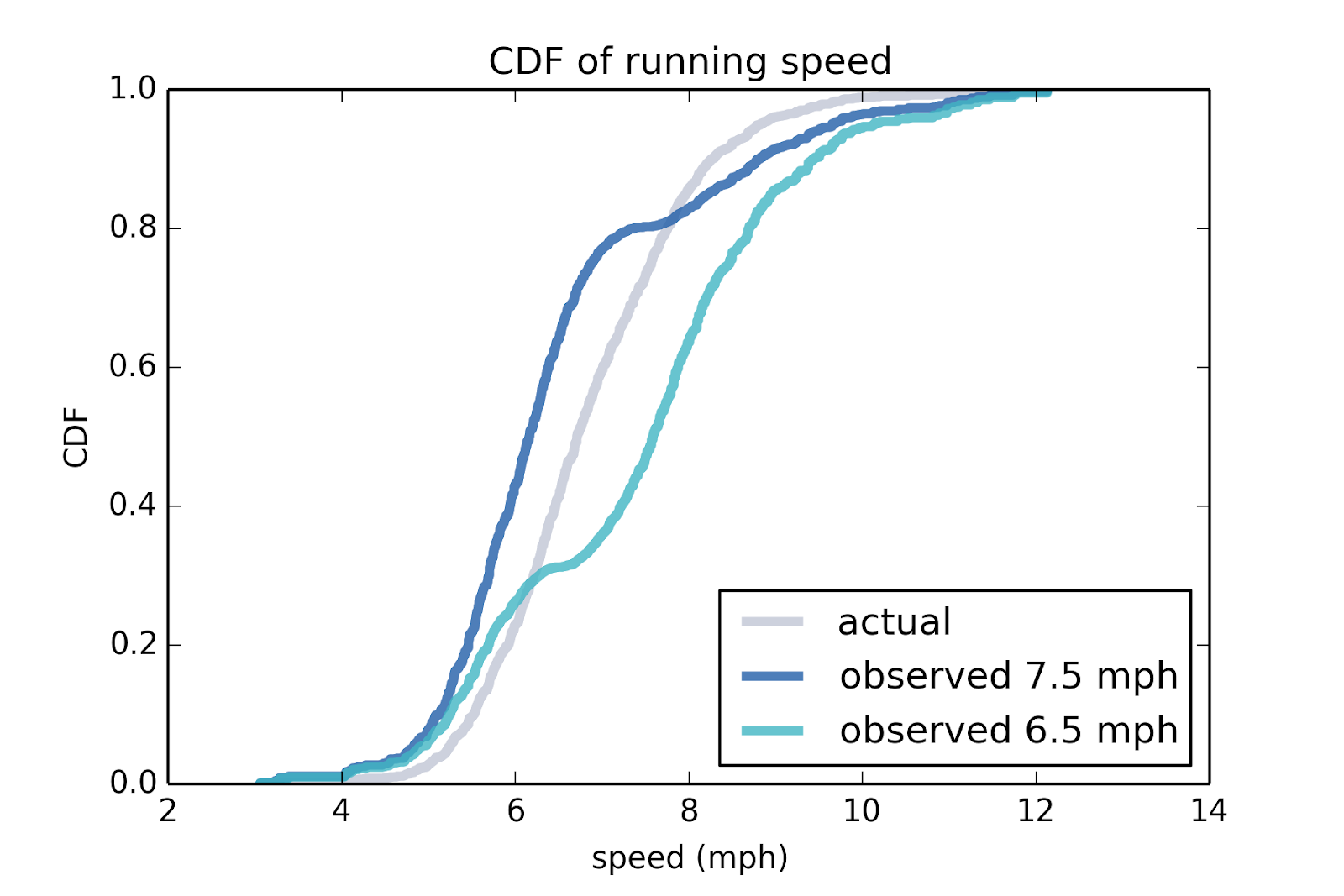
We can simulate this effect using data from a conventional road race.  Figure 4 shows the actual distribution of speeds from the James Joyce Ramble, a 10K race in Massachusetts.  It also shows biased distributions that would be seen by runners at 6.5 and 7.5 mph.  The observed distributions are bimodal, with fast and slow runners oversampled and fewer runners in the middle.
relay3.png
Figure 4: Distribution of speed for runners in a 10K, and biased distributions as seen by runners at different speeds.


A final example of the inspection paradox occurred to me when I was reading Orange is the New Black, a memoir by Piper Kerman, who spent 13 months in a federal prison.  At several points Kerman expresses surprise at the length of the sentences her fellow prisoners are serving.  She is right to be surprised, but it turns out that she is the victim of not just an inhumane prison system, but also the inspection paradox.


If you arrive at a prison at a random time and choose a random prisoner, you are more likely to choose a prisoner with a long sentence.  Once again, a prisoner with sentence x is oversampled by a factor of x.


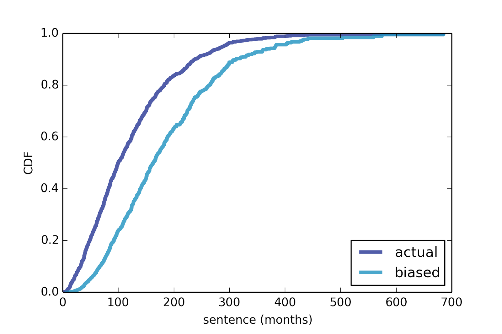
Using data from the U.S. Sentencing Commission, I made a rough estimate of the distribution of sentences for federal prisoners, shown in Figure 5.  I also computed the biased distribution as observed by a random arrival.
orange2.png
Figure 5: Approximate distribution of federal prison sentences, and a biased distribution as seen by a random arrival.


As expected, the biased distribution is shifted to the right.  In the actual distibution the mean is 121 months; in the biased distribution it is 183 months.


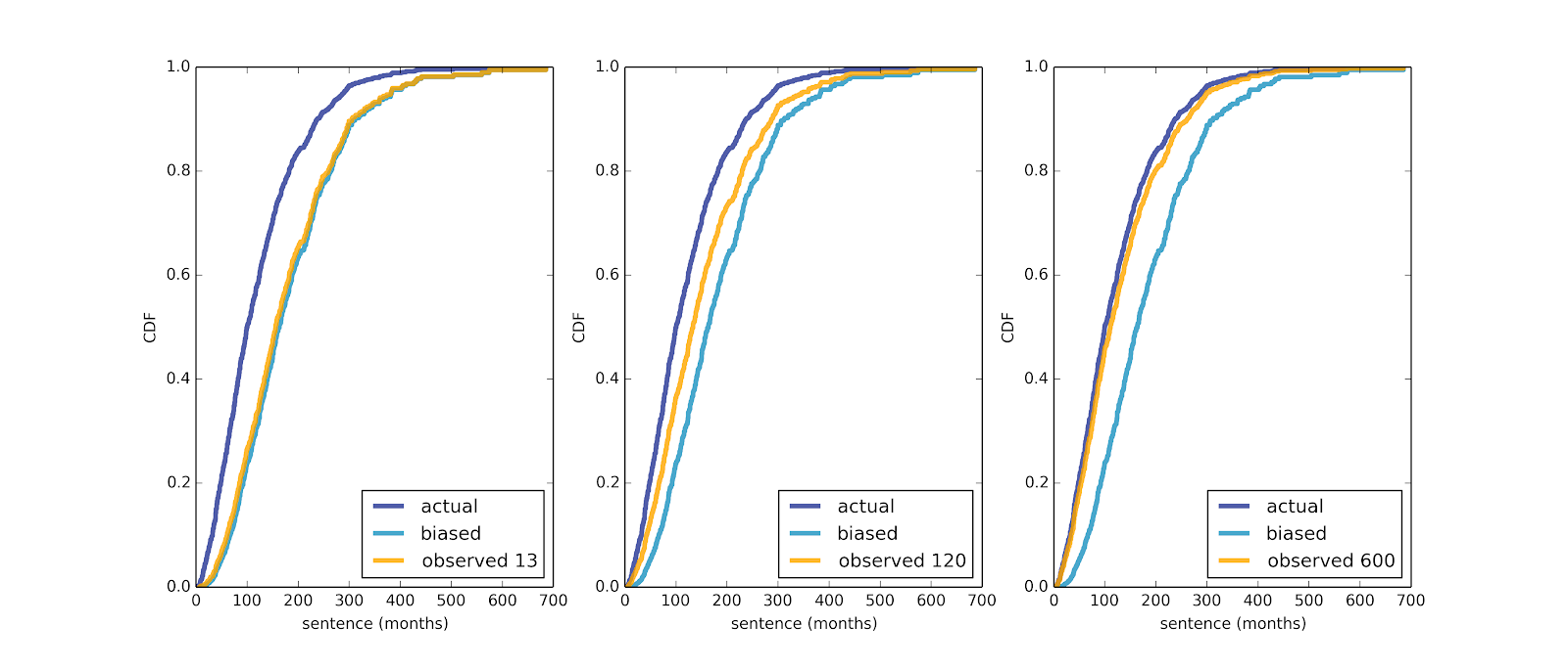
So what happens if you observe a prison over an interval like 13 months?  It turns out that if your sentence is y months, the chance of overlapping with a prisoner whose sentence is x months is proportional to x + y.


Figure 6 shows biased distributions as seen by hypothetical prisoners serving sentences of 13, 120, and 600 months.
orange6.png
Figure 6: Biased distributions as seen by prisoners with different sentences.


Over an interval of 13 months, the observed sample is not much better than the biased sample seen by a random arrival.  After 120 months, the magnitude of the bias is about halved.  Only after a very long sentence, 600 months, do we get a more representative sample, and even then it is not entirely unbiased.


These examples show that the inspection paradox appears in many domains, sometimes in subtle ways.  If you are not aware of it, it can cause statistical errors and lead to invalid inferences.  But in many cases it can be avoided, or even used deliberately as part of an experimental design.


Further reading
I discuss the class size example in my book, Think Stats, 2nd Edition, O’Reilly Media, 2014, and the Red Line example in Think Bayes, O’Reilly Media, 2013.  I wrote about relay races, social networks, and Orange Is the New Black in my blog, “Probably Overthinking It”.  http://allendowney.blogspot.com/


John Allen Paulos presents the friendship paradox in Scientific American, “Why You're Probably Less Popular Than Your Friends”, 18 January 2011.  http://www.scientificamerican.com/article/why-youre-probably-less-popular/
The original paper on the topic might be Scott Feld,  “Why Your Friends Have More Friends Than You Do”, American Journal of Sociology, Vol. 96, No. 6 (May, 1991), pp. 1464-1477. http://www.jstor.org/stable/2781907


Amir Aczel discusses some of these examples, and a few different ones, in a Discover Magazine blog article, “On the Persistence of Bad Luck (and Good)”, 4 September 4, 2013.


The code I used to generate these examples is in these Jupyter notebooks:


Bio

Allen Downey is a Professor of Computer Science at Olin College of Engineering in Massachusetts.  He is the author of several books, including Think Python, Think Stats, and Think Bayes.  He is a runner with a maximum 10K speed of 8.7 mph.

Tuesday, August 4, 2015

Orange is the new stat

I've been reading Piper Kerman's Orange Is the New Black, a memoir by a woman who served 11 months in a federal prison.  One of the recurring themes is the author's surprise at the length of the sentences her fellow prisoners are serving, especially the ones convicted of drug offences.  In my opinion, she is right to be shocked.

About half of federal prisoners were convicted of drug crimes, according to this fact sheet from the US Sentencing Commission (USSC).  In minimum security prisons, the proportion is higher, and in women's prisons, I would guess it is even higher.  About 45% of federal prisoners were sentenced under mandatory minimum guidelines that sensible people would find shocking.  And about a third of them had no prior criminal record, according to this report, also from the USSC.

In many cases, minor drug offenders are serving sentences much longer than sentences for serious violent crimes.  For a list of heart-breaking examples, see these prisoner profiles at Families Against Mandatory Minimums.

Or watch this clip from Jon Oliver's Last Week Tonight:


When you are done being outraged, here are a few things to do:

1) Read more about Families Against Mandatory Minimums, write about them on social media, and consider making a donation (Charity Navigator gives them an excellent rating).

2) Another excellent source of information, and another group that deserves support, is the Prison Policy Initiative.

3) Then read the rest of this article, which points out that although Kerman's observations are fundamentally correct, her sampling process is biased in an interesting way.

The inspection paradox

It turns out that Kerman is the victim not just of a criminal justice system that is out of control, but also of a statistical error called the inspection paradox.  I wrote about it in Chapter 3 of Think Stats, where I called it the Class Size Paradox, using the example of average class size.

If you ask students how big their classes are, the average of their responses will be higher than the actual average, often substantially higher.  And if you ask them how many children are in their families, the average of their responses will be higher than the average family size.

The problem is not the students, for once, but the sampling process.  Large classes are overrepresented in the sample because in a large class there are more students to report a large class size.  If there is a class with only one student, only one student will report that size.

And similarly with the number of children, large families are overrepresented and small families underrepresented; in fact, families with no children aren't represented at all.

The inspection paradox is an example of the Paradox Paradox, which is that a large majority of the things called paradoxes are not, actually, but just counter-intuitive truths.  The apparent contradiction between the different averages is resolved when you realize that they are averages over different populations.  One is the average in the population of classes; the other is the average in the population of student-class experiences.

Neither is right or wrong, but they are useful for different things.  Teachers might care about the average size of the classes they teach; students might care more about the average of the classes they take.

Prison inspection

The same effect occurs if you visit a prison.  Suppose you pick a random day, choose a prisoner at random, and ask the length of her sentence.  The response is more likely to be a long sentence than a short one, because a prisoner with a long sentence has a better chance of being sampled.  For each sentence duration, x, suppose the fraction of convicts given that sentence is p(x).  In that case the probability of observing someone with that sentence is proportional to x p(x).

Now imagine a different scenario: suppose you are serving an absurdly-long prison sentence, like 55 years for a minor drug offense.  During that time you see prisoners with shorter sentences come and go, and if you keep track of their sentences, you get an unbiased view of the distribution of sentence lengths.  So the probability of observing someone with sentence x is just p(x).

And that brings me to the question that occurred to me while I was reading Orange: what happens if you observe the system for a relatively short time, like Kerman's 11 months?  Presumably the answer is somewhere between p(x) and x p(x).   But where?  And how does it depend on the length of the observer's sentence?

UPDATE 17 August 2015: A few days after I posted the original version of this article, Jerzy Wieczorek dropped by my office.  Jerzy is an Olin alum who is now a grad student in statistics at CMU, so I posed this problem to him.  A few days later he emailed me the solution, which is that the probability of observing a sentence, x, during and interval, t, is proportional to x + t.  Couldn't be much simpler than that!

To see why, imagine a row of sentences arrange end-to-end along the number line.  If you make an instantaneous observation, that's like throwing a dart at the number line.  You chance of hitting a sentence with length x is (again) proportional to x.

Now imagine that instead of throwing a dart, you throw a piece of spaghetti with length t.  What is the chance that the spaghetti overlaps with a sentence of length x?  If we say arbitrarily that the sentence runs from 0 to x, the spaghetti will overlap the sentence if the left side falls anywhere between -t and x.  So the size of the target is x + t.

Based on this result, here's a Python function that takes the actual PMF and returns a biased PMF as seen by someone serving a sentence with duration t:

def bias_pmf(pmf, t=0):
    new_pmf = pmf.Copy()

    for x, p in pmf.Items():
        new_pmf[x] *= (x + t)
        
    new_pmf.Normalize()
    return new_pmf

This IPython notebook has the details, and here's a summary of the results.

Results

To model the distribution of sentences, I use random values from a gamma distribution, rounded to the nearest integer. All sentences are in units of months.  I chose parameters that very roughly match the histogram of sentences reported by the USSC.

The following code generates a sample of sentences as observed by a series of random arrivals.  The notebook explains how it works.

sentences = np.random.gamma(shape=2, scale=60, size=1000).astype(int)
releases = sentences.cumsum()
arrivals = np.random.random_integers(1, releases[-1], 10000)
prisoners = releases.searchsorted(arrivals)
sample = sentences[prisoners]
cdf2 = thinkstats2.Cdf(sample, label='biased')

The following figure shows the actual distribution of sentences (that is, the model I chose), and the biased distribution as would be seen by random arrivals:

Due to the inspection paradox, we oversample long sentences.  As expected, the sample mean is substantially higher than the actual mean, about 190 months compared to 120 months.

The following function simulates the observations of a person serving a sentence of t months.  Again, the notebook explains how it works:

def simulate_sentence(sentences, t):
    counter = Counter()
    
    releases = sentences.cumsum()
    last_release = releases[-1]
    arrival = np.random.random_integers(1, max(sentences))
    
    for i in range(arrival, last_release-t, 100):
        first_prisoner = releases.searchsorted(i)
        last_prisoner = releases.searchsorted(i+t)
    
        observed_sentences = sentences[first_prisoner:last_prisoner+1]
        counter.update(observed_sentences)
    
    print(sum(counter.values()))
    return thinkstats2.Cdf(counter, label='observed %d' % t)

Here's the distribution of sentences as seen by someone serving 11 months, as Kerman did:


The observed distribution is almost as biased as what would be seen by an instantaneous observer.  Even after 120 months (near the average sentence), the observed distribution is substantially biased:

After 600 months (50 years!) the observed distribution nearly converges to the actual distribution.

I conclude that during Kerman's 11 month sentence, she would have seen a biased sample of the distribution of sentences.  Nevertheless, her observation  that many prisoners are serving long sentences that do not fit their crimes  is still valid, in my opinion.