This article presents a "one-day paper", my attempt to pose a research question, answer it, and publish the results in one work day (May 13, 2016).
Copyright 2016 Allen B. Downey
MIT License: https://opensource.org/licenses/MIT
from __future__ import print_function, division

from thinkstats2 import Pmf, Cdf

import thinkstats2
import thinkplot

import pandas as pd
import numpy as np
from scipy.stats import entropy

%matplotlib inline
What's a generation supposed to be, anyway?
If generation names like "Baby Boomers" and "Generation X" are just a short way of referring to people born during certain intervals, you can use them without implying that these categories have any meaningful properties.
But if these names are supposed to refer to generations with identifiable characteristics, we can test whether these generations exist. In this notebook, I suggest one way to formulate generations as a claim about the world, and test it.
Suppose we take a representative sample of people in the U.S., divide them into cohorts by year of birth, and measure the magnitude of the differences between consecutive cohorts. Of course, there are many ways we could define and measure these differences; I'll suggest one in a minute.
But ignoring the details for now, what would those difference look like if generations exist? Presumably, the differences between successive cohorts would be relatively small within each generation, and bigger between generations.
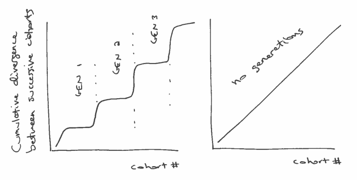
If we plot the cumulative total of these differences, we expect to see something like the figure below (left), with relatively fast transitions (big differences) between generations, and periods of slow change (small differences) within generations.
On the other hand, if there are no generations, we expect the differences between successive cohorts to be about the same. In that case the cumulative differences should look like a straight line, as in the figure below (right):
So, how should we quantify the differences between successive cohorts. When people talk about generational differences, they are often talking about differences in attitudes about political, social issues, and other cultural questions. Fortunately, these are exactly the sorts of things surveyed by the General Social Survey (GSS).
To gather data, I selected question from the GSS that were asked during the last three cycles (2010, 2012, 2014) and that were coded on a 5-point Likert scale.
You can see the variables that met these criteria, and download the data I used, here:
https://gssdataexplorer.norc.org/projects/13170/variables/data_cart
Now let's see what we got.
First I load the data dictionary, which contains the metadata:
dct = thinkstats2.ReadStataDct('GSS.dct')
Then I load the data itself:
df = dct.ReadFixedWidth('GSS.dat')
I'm going to drop two variables that turned out to be mostly N/A
df.drop(['immcrime', 'pilloky'], axis=1, inplace=True)
And then replace the special codes 8, 9, and 0 with N/A
df.ix[:, 3:] = df.ix[:, 3:].replace([8, 9, 0], np.nan)
df.head()
For the age variable, I also have to replace 99 with N/A
df.age.replace([99], np.nan, inplace=True)
Here's an example of a typical variable on a 5-point Likert scale.
thinkplot.Hist(Pmf(df.choices))

I have to compute year born
df['yrborn'] = df.year - df.age
Here's what the distribution looks like. The survey includes roughly equal numbers of people born each year from 1922 to 1996.
pmf_yrborn = Pmf(df.yrborn)
thinkplot.Cdf(pmf_yrborn.MakeCdf())

Next I sort the respondents by year born and then assign them to cohorts so there are 200 people in each cohort.
df_sorted = df[~df.age.isnull()].sort_values(by='yrborn')
df_sorted['counter'] = np.arange(len(df_sorted), dtype=int) // 200
df_sorted[['year', 'age', 'yrborn', 'counter']].head()
df_sorted[['year', 'age', 'yrborn', 'counter']].tail()
I end up with the same number of people in each cohort (except the last).
thinkplot.Cdf(Cdf(df_sorted.counter))
None

Then I can group by cohort.
groups = df_sorted.groupby('counter')
I'll instantiate an object for each cohort.
class Cohort:
    skip = ['year', 'id_', 'age', 'yrborn', 'cohort', 'counter']

    def __init__(self, name, df):
        self.name = name
        self.df = df
        self.pmf_map = {}

    def make_pmfs(self):
        for col in self.df.columns:
            if col in self.skip:
                continue
            self.pmf_map[col] = Pmf(self.df[col].dropna())
            try:
                self.pmf_map[col].Normalize()
            except ValueError:
                print(self.name, col)

    def total_divergence(self, other, divergence_func):
        total = 0
        for col, pmf1 in self.pmf_map.items():
            pmf2 = other.pmf_map[col]
            divergence = divergence_func(pmf1, pmf2)
            #print(col, pmf1.Mean(), pmf2.Mean(), divergence)
            total += divergence
        return total
To compute the difference between successive cohorts, I'll loop through the questions, compute Pmfs to represent the responses, and then compute the difference between Pmfs.
I'll use two functions to compute these differences. One computes the difference in means:
def MeanDivergence(pmf1, pmf2):
    return abs(pmf1.Mean() - pmf2.Mean())
The other computes the Jensen-Shannon divergence
def JSDivergence(pmf1, pmf2):
    xs = set(pmf1.Values()) | set(pmf2.Values())
    ps = np.asarray(pmf1.Probs(xs))
    qs = np.asarray(pmf2.Probs(xs))
    ms = ps + qs
    return 0.5 * (entropy(ps, ms) + entropy(qs, ms))
First I'll loop through the groups and make Cohort objects
cohorts = []
for name, group in groups:
    cohort = Cohort(name, group)
    cohort.make_pmfs()
    cohorts.append(cohort)

len(cohorts)
Each cohort spans a range about 3 birth years. For example, the cohort at index 10 spans 1965 to 1967.
cohorts[11].df.yrborn.describe()
Here's the total divergence between the first two cohorts, using the mean difference between Pmfs.
cohorts[0].total_divergence(cohorts[1], MeanDivergence)
And here's the total J-S divergence:
cohorts[0].total_divergence(cohorts[1], JSDivergence)
This loop computes the (absolute value) difference between successive cohorts and the cumulative sum of the differences.
res = []
cumulative = 0
for i in range(len(cohorts)-1):
    td = cohorts[i].total_divergence(cohorts[i+1], MeanDivergence)
    cumulative += td
    print(i, td, cumulative)
    res.append((i, cumulative))
The results are a nearly straight line, suggesting that there are no meaningful generations, at least as I've formulated the question.
xs, ys = zip(*res)
thinkplot.Plot(xs, ys)
thinkplot.Config(xlabel='Cohort #',
                ylabel='Cumulative difference in means',
                legend=False)

The results looks pretty much the same using J-S divergence.
res = []
cumulative = 0
for i in range(len(cohorts)-1):
    td = cohorts[i].total_divergence(cohorts[i+1], JSDivergence)
    cumulative += td
    print(i, td, cumulative)
    res.append((i, cumulative))
xs, ys = zip(*res)
thinkplot.Plot(xs, ys)
thinkplot.Config(xlabel='Cohort #',
                ylabel='Cumulative JS divergence',
                legend=False)

Conclusion: Using this set of questions from the GSS, and two measures of divergence, it seems that the total divergence between successive cohorts is nearly constant over time.
If a "generation" is supposed to be a sequence of cohorts with relatively small differences between them, punctuated by periods of larger differences, this study suggests that generations do not exist.
Interesting approach! My first instinct would have been to plot age on the x-axis and an index of social and political attitudes on the y-axis, fit a spline, and examine jumps at the lower and upper bounds of each generational interval. I wonder if this would produce different results.
ReplyDeleteIf it did, how would you reconcile it with the results of this analysis?
DeleteGood questions. What I have done so far is one attempt to find a generational effect, which failed. So there could still be an effect, but my experiment missed it.
ReplyDeleteI am planning a follow-up that will try harder to show the effect, by searching specifically for questions that show a generational pattern and aggregating them.
Watch this space.