Thursday, February 24, 2011

Moving the goalposts

Last week I wrote about the effect of the Boston Marathon qualifying standard on finish times in other marathons.  The next day the organizers of the Boston Marathon, the BAA, announced new qualifying standards for 2012 and 2013 and a new registration process.  Here is my summary of the announcement:

  • For 2012, qualifying times for all groups are lower by 1 minute.
  • For 2013, qualifying times for all groups drop another 5 minutes.
  • For both years, runners who beat their qualifying time by 20 minutes are allowed to register first, followed by runners who qualify by 10 minutes, 5 minutes, and then 0 minutes.

Among runners, there has been a lot of discussion of the effect these changes will have on the demographics of the race, especially the proportion of women and older runners.

To answer this question, we have to get a sense of what the pool of potential qualifiers looks like.  I collected data from the 2008, 2009 and 2010 Chicago Marathons (don’t ask me how).  This dataset includes 101135 finish times with the gender and age of each runner.  To keep things simple, I treat each finish time as a different runner, even though many people ran the race in more than one of the years I looked at.

I selected runners in the 18-34 group, which includes 22619 men and 24471 women.  Then I selected the runners who ran 30 minutes over the current qualifying standard or faster, which includes 4951 men and 5502 women.

For each finish time, I computed the difference between the actual time and the standard (3:10 for men, 3:40 for women).  This figure shows the distribution of those differences:


The BQ Effect, which I wrote about last week, is apparent for men and women.  For the men there is another mode 10 minutes below the standard, which happens to be 3:00:00.  Apparently the only thing more important than qualifying for Boston is breaking 3 hours.

The runners in this dataset are a sample of the population that constitutes the field at Boston.  If we assume that this sample is representative, we can use it to predict the effect of the changes in the qualifying standard.

As a baseline, in 2010 there were 9602 finishers in the open division, 4651 men and 4951 women.  In the Chicago sample, tightening the standard by 1 minute (which will happen in 2012) disqualifies 92 men (4.9%) and 102 women (5.6%).  Extrapolating these changes to the open division in Boston (9602), the net effect is to replace 16 women with men.

In 2013, the standard will be 6 minutes lower, which disqualifies 30.1% of men and 33.9% of women, and displaces 134 women.

The new registration process might make the effect even more dramatic.  If the field fills before the last group has a chance, the standard is effectively tougher by 11 minutes.  That disqualifies 41.6% of men, 50.5% of women, and displaces 395 women.

This change would be noticeable.  In 2010, the open division was almost 52% female.  In 2013, it might be 52% male.

Is that fair?  I will argue that it is not, but it will take some time to make the argument clear.  Let me start by explaining why some people think it’s fair.  It is conventional wisdom that the current standard is relatively easy for women.  If that’s true, then these changes will be a correction.

For example, in this article Amby Burfoot proposes a standard based on the age-graded tables created by World Masters Athletics (WMA).  Under that standard, the qualifying times would be 3:12 for men and 3:30 for women.  In the Chicago sample, that would increase the number of men by 8% and decrease the number of women by 47%.  Extrapolating to Boston, it would replace 1751 women with men, yielding a field of 66% men.

I think this standard is unreasonable because the WMA tables are based on world records in each group, not the performance of more typical qualifiers.  The proposed standard has a bigger effect on women because the elite females are farther from the pack than the elite males.

To see the the tail of the distribution, let’s zoom in on the runners in the Chicago sample who beat the standard by 30 minutes or more:


The tail for women extends farther to the left.  The fastest men beat the standard by 65 minutes; the fastest women beat it by more than 80 minutes.  But the existence of a small number of outliers should not have such a drastic effect on the qualifying standard.

In conclusion:

1) The changes in the qualifying standard and process might decrease the representation of women in Boston from 52% to 48%.

2) The common belief that the standard is relatively easy for women is based on the performance of a small number of outliers.  The gender gap for near-qualifiers is much larger than the gap for elites.

3) Implementing the standard proposed by Runners’ World would decrease the percentage of women in the open division at Boston to 33%.

-----

Coming soon:

1) I will evaluate possible definitions of a “fair” standard and compute qualifying times for each definition.

2) I will extend this analysis to the other age groups.

-----


If you find this sort of thing interesting, you might like my free statistics textbook, Think Stats. You can download it or read it at thinkstats.com.

Monday, February 14, 2011

The BQ Effect

In order to register for the Boston Marathon, you have to run another marathon faster than the qualifying standard for your age group and gender.  For example, men 34 and under have to run 3:10 or better.  Since I am 43, my qualifying time is 3:20 -- on my 45th birthday I get another ten minutes (wrapped up with a bow).

These standards are challenging.  At most major marathons, less than 20% of the field runs a Boston qualifying time, known as a “BQ.”  According to marathonguide.com, the races in 2010 with the highest percentage of qualifiers were the Bay State Marathon (37%) and Boston itself (44%).

Two years ago I ran the Bay State Marathon in my first (unsuccessful) attempt to qualify.  I was almost on pace for the first 20 miles, then hit the wall and slowed from 7:50 per mile to 10:00.  While I shuffling through the last few miles, I wondered whether the Boston qualifying times have a visible effect on the distribution of finish times.

I can imagine several possible BQ effects: (1) an excess of runners finishing just under the qualifying time, (2) a deficit of runners just over, and maybe (3) an excess of runners like me who attempt a qualifying time, bonk, and end up 10-20 minutes over.

To look for these effects, I collected data from the 2010 Bay State Marathon (available at coolrunning.com).  For each of the 1564 finishers, I looked up their age and gender to get qualifying times, and computed the difference in minutes between their actual and qualifying times.

For comparison, I also collected data from the 2010 Sun Lowell Half Marathon, which runs on (mostly) the same course at the same time.  For each half-marathoner, I computed a marathon time prediction using the well-known Riegel formula.

The following figure shows the PMF of finish time, relative to qualifying time, for runners in both races whose finish time (real or imagined) was within 60 minutes of their qualifying time.  A negative difference means the runner qualified.


As expected, there is a substantial mode just under the qualifying time for the marathoners, but not for the half marathoners.  The other two hypothetical effects are not apparent.

PMFs tend to be noisy, so I generally prefer to look at CDFs:


Again, the BQ effect is clear: in the full marathon there are more runners just under the qualifying time and fewer just over.  But either the number of people who bonk is small, or their times are sufficiently spread out that they don’t constitute an apparent mode.  I am a mode of one.

-----


If you find this sort of thing interesting, you might like my free statistics textbook, Think Stats. You can download it or read it at thinkstats.com.

Monday, February 7, 2011

Are first babies more likely to be late?

UPDATE: The version of this article with the most recent data is here.


When my wife and I were expecting our first child, we heard from several people that first babies tend to be late.  If you Google this question, you will find plenty of discussion.  Some people claim it's true, others say it's a myth, and some people say it's the other way around: first babies come early.

What you will probably not find is any data to support these claims.  Except this kind of data:
``My two friends that have given birth recently to their first babies, BOTH went almost 2 weeks overdue before going into labour or being induced.''

``I don't think that can be true because my sister was my mother's first and she was early, as with many of my cousins.''
If you don’t find those arguments compelling, you might be interested in the National Survey of Family Growth (NSFG), a survey conducted by the U.S. Centers for Disease Control and Prevention (CDC) to gather ``information on family life, marriage and divorce, pregnancy, infertility, use of contraception, and men's and women's health.”

Their 2002 dataset includes 7643 women, who reported the gestational age for their 9148 live births.  This figure shows the distribution of pregnancy length:


The distributions are similar for first babies and others.  The mode is 39 weeks; the distribution is skewed to the left, with some births as early as 24 weeks, but almost none later than 44 weeks.

On average, first babies are 0.078 weeks later than others.  This difference, 13 hours, is not statistically significant.  But there are differences in the shape of the distribution.  This figure shows the percent difference between first babies and others for weeks 34 through 46:


The general pattern is that first babies are more likely to be early (37 weeks or less), less likely to be on time (38-40), and more likely to be late (41 or more).  In terms of relative risk, first babies are 8% more likely to be born early and 66% more likely to be late.  And those differences are statistically significant (using a chi-square test, p < 0.001).

So far, none of this is useful for planning, so let’s consider a scenario: suppose you are in week 38 and you want to know your chances of delivering during the next three weeks.  For first babies, the chance is 81%, for others it is 89%.  So yes, in this scenario, first babies are more likely to be late.  Sorry.


Wednesday, February 2, 2011

Yet another reason SAT scores are non-predictive

Most colleges use the SAT as a criterion for admission because they assume that SAT scores contain information about students’ preparation.  The College Board defends this assumption with evidence that SAT scores are correlated with first-year college grades.  But even in their own studies, the correlation is only R=0.53.

Correlations are often reported in terms of “explained variability”: a correlation of 0.53 explains R^2=28% of the variance in the data.  But even that overstates the predictive power of SAT scores because it is expressed in terms of variance, not standard deviation.

To make that more concrete, suppose you are trying to guess students’ first year grades; how much better could you guess if you knew their SAT scores?  Without using SAT scores, the best you could do is to guess the mean, which is 2.97 in the College Board study.  In that case your root-mean-squared-error (RMS) would be the standard deviation, 0.71.

Using SAT scores, you could reduce RMS to 0.60, which is a 15% improvement.  That’s a little bit better, but 0.6 is the difference between a B average and an A-, and you should expect to be off by at least that much 32% of the time.

At colleges with strict admissions standards, the correlation tends to be even lower.  There are two reasons for this effect.  One is explained in this article by John Allen Paulos, who points out that “Colleges usually accept students from a fairly narrow swath of the SAT spectrum,” and “the degree of correlation between two variables depends on the range of the variables considered.”

To see why that’s true, consider Harvard, where the 25th percentile for the combined SAT is 2100 (see satscores.us).  So 75% of the students averaged 700 or better on the three parts of the exam.  That’s a “fairly narrow swath.”

In fact the problem is even worse than Paulos suggests, because the SAT doesn’t discriminate very well between people at the top of the scale.  For example, the difference between a 700 and a 770 can be as few as 4 questions, which might be due to chance.

To quantify that, I will compute the chance that someone who gets a 700 is actually better than someone with an 770.  By “better,” I only mean “better at answering SAT questions,” which I will describe with P, the probability of getting a question right.

To estimate a student’s value of P, we start with a prior distribution and use the test score to perform an update.  We can get a reasonable prior distribution by taking the distribution of scaled scores, mapping them back to raw scores, and converting raw scores to percentages.

I got the distribution of scores and the scale from College Board data tables.  The distribution of raw scores is roughly normal (by design).  This figure shows a normal probability plot, which compares the actual values to random values from a normal distribution:


The red line shows a linear fit to the data.  At both ends, the data deviate from the model, which indicates that the range of the test is not as wide as the range of ability; if it were, the top score would be 80, not 54.

Nevertheless, we can convert these scores to percentages (54/54 = 100%) and use the distribution of percentages as a prior for P.  Then to perform a Bayesian update, we compute the likelihood of a score, R, given P:

def Likelihood(self, R, P):
    right = R
    wrong = 54 - R
    return pow(P, right) * pow(1-P, wrong)

Which is an unnormalized binomial probability.  This figure shows the posterior distributions of P for hypothetical students with scores of 700 and 770:


The 90% credible interval for a student who gets a 700 is (650, 730); for a student who gets a 770 it is (700, 780).  To put that in perspective, at Harvard the interquartile range for the math exam is 700-790.  So a student who gets a 770 might really be in the 25th percentile of his or her class.  And the chance is about 10% that a classmate who got a 700 is actually better (at answering SAT questions, anyway).

-----

Notes: I made some simplifications, all of which tend to underestimate the margin of error for SAT scores.

1) Some SAT questions are easier than others, so the probability of getting each question is not the same.  For students at the top of the range, the probability of getting the easy questions is close to 1, so the observed differences are effectively based on a small number of more difficult questions.

2) The compression of scores at the high end also compresses the margins of error.  For example, the credible interval for a student who gets a 770 only goes up to 780.  This is clearly an underestimate.

3) I ignored the fact that students who miss a question lose ¼ point.  Since students at the top end of the range usually answer every question, a student who missed 4 questions loses 5 points, amplifying the effect of random errors.

Monday, January 24, 2011

Are you popular? Hint: no.

According to this feel-good article in Scientific American, you are probably less popular than your friends.  The author, John Allen Paulos, explains:

“...it’s more probable that we will be among a popular person’s friends simply because he or she has a larger number of them.”

The same logic explains the class size paradox I wrote about in Think Stats.  If you ask students how big their classes are, more of them will report large classes, because more of them are in large classes.

To see how this works in social networks, I downloaded data from the Stanford Large Network Dataset Collection; one of the datasets there contains friend/foe information from the Slashdot Zoo.  For each (anonymized) user, we have the number of other users he or she tagged as a friend or foe.

There are more than 82,000 users in the dataset.  The average user has 55 friends and foes, but the median is only 18, which suggests that the distribution is skewed to the right.  In fact, the distribution is heavy tailed, as shown in the figure below.


The blue line is the distribution for a randomly-chosen user.  As expected, it is right-skewed, even on a log scale.  Most people have fewer than 20 connections, but 15% have more than 100 and 0.2% have more than 1000.

The green line is the distribution for your friends.  It is biased because more popular people are more likely to be your friend.  In the extremes, a person with no friends has no chance to be your friend; a person with thousands of friends has a much higher probability.  In general, a person with n friends is n times more likely than a person with 1 friend.

So if we choose a person at random, and then choose one of their friends at random, we get the biased distribution.  The difference is substantial, about an order of magnitude.  In the biased distribution, the mean is 308, the median 171.  So what are the chances that your friend is more popular than you?  In this distribution, about 84%.

Loser.

-----

To compute the biased distribution, we loop through the items in the PMF and multiply each probability by its corresponding value.  Here’s what the code looks like:


def BiasPmf(pmf, name, invert=False):
   """Returns the Pmf with oversampling proportional to value.

   If pmf is the distribution of true values, the result is the
   distribution that would be seen if values are oversampled in
   proportion to their values; for example, if you ask students
   how big their classes are, large classes are oversampled in
   proportion to their size.

   If invert=True, computes the inverse operation; for example,
   unbiasing a sample collected from students.

   Args:
     pmf: Pmf object.
     invert: boolean

    Returns:
      Pmf object
   """
   new_pmf = pmf.Copy()
   new_pmf.name = name

   for x, p in pmf.Items():
       if invert:
           new_pmf.Mult(x, 1.0/x)
       else:
           new_pmf.Mult(x, x)
       
   new_pmf.Normalize()
   return new_pmf


Monday, January 17, 2011

Obesity epidemic cured!


I have good news to report -- the obesity epidemic is over.  And the solution turns out to be the best kind: simple and completely painless.  The solution is self-reporting.  Instead of weighing people, all we have to do is ask them what they weigh.  Problem solved!

I got data from the Behavioral Risk Factor Surveillance System (BRFSS), run by the National Center for Chronic Disease Prevention and Health Promotion.  In 2008, they surveyed 414,509 respondents and asked about their demographics, health and health risks.  In particular, they asked respondents for their weight now and their weight one year ago.

By taking the difference, we can characterize weight change in the population.  And the news is good.  According to these reports, the average weight change was -0.64 kilos; that is, the average respondent lost 1.4 pounds.

Of course, this result is unrelated to reality.  In fact, most adults gain about a pound a year.  The most likely explanation is some combination of inaccurate recall, self-delusion, and attempts by respondents to impress surveyors.

But before making harsh judgments, let’s look more closely at the data.  Before computing the mean change, I discarded a few outliers -- anyone who reported a change of more than 40 kg.  Even so, the mean can be misleading, so we should look at the distribution.  This figure shows the cumulative distribution (CDF) of reported weight changes:


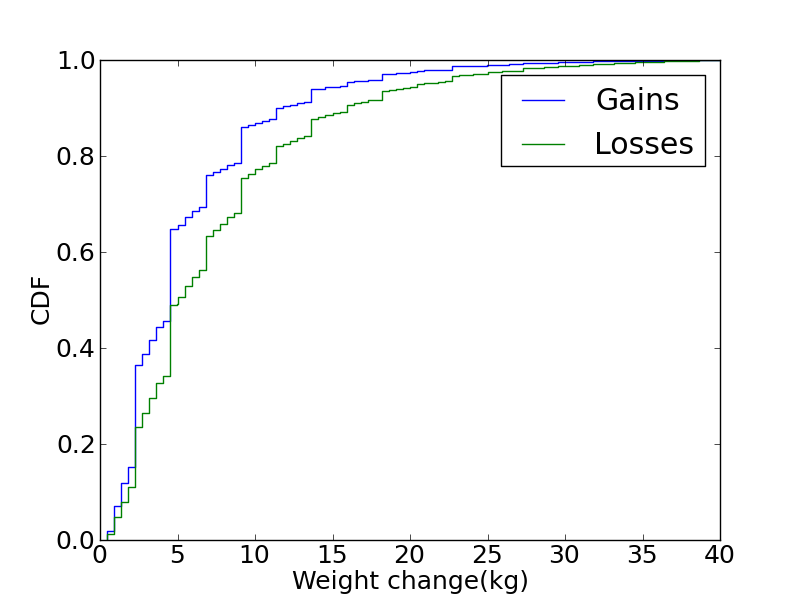
About 25% of respondents reported a weight loss, 52% reported no change, and 23% reported a gain.  The distribution is roughly symmetric, but we can get a better look by plotting CDFs for gains and losses:


The curves have the same shape, but the distribution of losses is shifted to the right.  This result suggests that we can’t blame a small number of wildly inaccurate respondents; delusion seems to be widespread.

These data demonstrate the dangers of self-reporting.  Even when surveys are administered carefully, people tend to remember wrongly, kid themselves, and portray themselves in a positive light.

But if you want the obesity epidemic to go away, just ask!

----------


If you are interested in topics like this, you might like my book, Think Stats: Probability and Statistics for Programmers.

Monday, January 10, 2011

Observer effect in relay races

In most foot races, everyone starts at the same time.  If you are a fast runner, you usually pass a lot of people at the beginning of the race, but after a few miles everyone around you is going at the same speed.

Last September I ran the Reach the Beach relay, where teams of 12 run 209 miles in New Hampshire from Cannon to Hampton Beach.  While I was running my second leg, I noticed an odd phenomenon: when I overtook another runner, I was usually much faster, and when other runners overtook me, they were usually much faster.

At first I thought that the distribution of speeds might be bimodal; that is, there were many slow runners and many fast runners, but few at my speed.  Then I realized that I was the victim of selection bias.

The race was unusual in two ways: it used a staggered start, so teams started at different times; also, many teams included runners at different levels of ability.  As a result, runners were spread out along the course with little relationship between speed and location.  When I started my leg, the runners near me were (pretty much) a random sample of the runners in the race.

So where does the bias come from?  During my time on the course, the chance of overtaking a runner, or being overtaken, is proportional to the difference in our speeds.  To see why, think about the extremes.  If another runner is going at the same speed as me, neither of us will overtake the other.  If someone is going so fast that they cover the entire course while I am running, they are certain to overtake me.

To see what effect this has on the distribution of speeds, I downloaded the results from a race I ran last spring (the James Joyce Ramble 10K in Dedham MA) and converted the pace of each runner to MPH.  Here’s what the probability mass function (PMF) of speeds looks like in a normal road race (not a relay):


It is bell-shaped, which suggests a Gaussian distribution.  There are more fast runners than we would expect in a Gaussian distribution, but that’s a topic for another post.

Now, let’s see what this looks like from the point of view of a runner in a relay race going 7.5 MPH.  For each speed, x, I apply a weight proportional to abs(x-7.5).  The result looks like this:


It’s bimodal, with many runners faster and slower than the observer, but few runners at or near the same speed.  So that’s consistent with my observation while I was running.  (The tails are spiky, but that’s an artifact of the small sample size.  I could apply some smoothing, but I like to keep data-mangling to a minimum.)

One of the nice things about long-distance running is that you have time to think about things like this.

-----

Appendix: Here’s the code I used to compute the observed speeds:

def BiasPmf(pmf, speed, name=None):
    """Returns a new PDF representing speeds observed at a given speed.


    The chance of observing a runner is proportional to the difference in speed.


    Args:
        pmf: distribution of actual speeds
        speed: speed of the observing runner
        name: string name for the new dist


    Returns:
        Pmf object
    """
    new = pmf.Copy(name=name)
    for val, prob in new.Items():
        diff = abs(val - speed)
        new.Mult(val, diff)
    new.Normalize()
    return new


This code uses the PMF library, which you can read about in my book, Think Stats.